Generation of Three-Dimensional Image of Objects Submerged in Murky Water

Generación de imagen tridimensional de objetos sumergidos en aguas turbias

David J. Muñoz¹
George Archbold¹
Geraldine Delgado¹
Leydi V. Muñoz²
Juan Contreras¹

Abstract

This article presents the design and implementation of a novel method to generate 3D coordinates from the projection of a laser line over a solid object and the processing of the images obtained during scanning. The result obtained is a 3D model of an isometric view that provides the possibility of being seen from different perspectives under a virtual environment. The methodology is applied in the capture and reconstruction of 3D images of objects submerged in murky waters.

Key words: three-dimensional digitizing, triangulation, thresholding, skelotonization, rendering

Resumen

Este artículo presenta el diseño e implementación de un novedoso método para generar coordenadas tridimensionales a partir de la proyección de una línea láser sobre un objeto sólido y el procesamiento de las imágenes obtenidas durante el escaneo. El resultado obtenido es un modelo tridimensional de una vista isométrica que brinda la posibilidad de ser visto desde diferentes perspectivas bajo un ambiente virtual. La metodología es aplicada en la captura y reconstrucción de imágenes tridimensionales de objetos sumergidos en aguas turbias.

Palabras claves: digitalización tridimensional, triangulación, umbralización, esqueletización, renderización.

Date Received: December 13th, 2012 - Fecha de recepción: 13 de Diciembre de 2012
Date Accepted: March 4th, 2013 - Fecha de aceptación: 4 de Marzo de 2013

________________________

¹Escuela Naval Almirante Padilla. Facultad de Ingeniería Naval. Cartagena de Indias, Colombia. e-mail: daviermual@hotmail.com,
gw.archbold@ gmail.com, geraldine_delgado@hotmail.com, epcontrerasj@ieee.org
²Universidad del Cauca. Facultad de Ingeniería. Popayán, Colombia. e-mail: vivianarobles@unisoftcolombia.com
............................................................................................................................................................

Introduction

One of the main objectives of underwater vehicles is to navigate and inspect underwater environments autonomously. To improve the performance of those tasks, the vehicle must have efficient systems to collect and process information from the environment, which it receives through different types of sensors. Sonar is fundamental in this process and provides high-resolution images of the submarine scene; however, those images are not easy to process automatically and are generally accompanied by significant levels of noise.

Some underwater vehicles used for ship hull inspection, like the Hovering Autonomous Underwater Vehicles (HAUV), have Doppler Velocity Log (DVL) recorders to accomplish adequate control and navigation parallel to the hull; however, the DVL cannot be used to navigate and inspect in complex regions, like the propellers or rudder, which require the use of sonar and which is also used to construct 3D images from the data collected (Dema, 2006).

One of the most important developments worldwide has been the HAUV, which was designed and constructed jointly by Bluefin Robotics and MIT (Vaganay, 2006a; 2006b). The HAUV employs a Doppler velocity log-type sensor for control and navigation parallel to the hull line that also permits maintaining the sonar within the estimated operation range without external aid and without the need to previously prepare the ship’s surface.

Seebyte Ltd., located in Edinburgh, Scotland, made an important modification to the HAUV by adding a Dual Frequency Identification Sonar (DIDSON) (Reed et al., 2006). The fusion of the information from the DVL and the DIDSON permitted, through complex algorithms, reconstructing 3D images from complex zones like the propeller and rudder.

Another important development has been the ship hull automatic inspection system designed and constructed by Desert Star Systems, which it has denominated AquaMap (2006) and consists of an acoustic positioning system that generates a two dimensional image of the ship’s hull. The AquaMap does not have an automatic positioning system; rather, it requires for its operation four guide lines placed on the ship’s lowest side to serve as reference points.

To generate 3D images of the ship’s hull, information from consecutive sonar needs to be processed through complex algorithms that permit eliminating errors due to image noise. Other techniques do not use sonar and focus on maintaining the camera viewing angle parallel to the surface of the ship hull by using laser pointers, controlled inclination platforms, and Cartesian platforms. These use laser triangulation techniques to improve precision (Caccia, 2007; Zainal, 2007).

Digitizing 3D Images

The fundamental aspect of implementing digitizing systems lies on the possibility of reproducing geometries of existing objects. This is especially useful in complex objects in terms of their shapes, contours, and profiles.

Distinct 3D digitizing systems exist, which can be mainly divided into two big groups: digitizing through contact and digitizing without contact. The main advantage of 3D digitizers without contact is that they have a higher rate of data acquisition than digitizers with contact. We can divide the digitizing techniques without contact into two: the stereoscopic or passive vision methods, where the scene being analyzed is not interfered; and active vision methods, where some type of action is undertaken on the scene, whether it is through its illumination or by sending an energy beam (Montalvo, 2010).

The active vision technique was selected because these systems only require a light emitter (laser) and a receptor (camera) to obtain x, y, and z coordinates of each point of the object to reconstruct. The technique consists in that knowing the direction of the beam emitted and that of the beam received, the dimensions of the triangle are obtained and, hence, the depth of the point inspected. The following elements were used to apply the technique elected:

• High-resolution color TV submarine camera (600 TVL): 600-line horizontal resolution; effective pixels: PAL 795x596; minimum illumination of 0.00035 lux; 66° angle coverage; power: 12 Vdc/80 mA; video connection: 1 BNC 1Vp-p (75 ohm); operational depth: 200 m.
• Line generating laser: 532-nm wavelength; A/R coated crystal lens (adjustable focus); 1.4-mrad divergence; 65-mm length; 16-mm diameter.

Using a line generating laser permitted obtaining a large amount of pixels representative of the profile to reconstruct in a single take. If a pointer laser had been used, it would have to be projected a great many times to obtain this same information. This technique used permitted the calculation of the position (x, y, and z coordinates) of each pixel to be processed in parallel manner for a single image, thus, reducing image processing times.

Reconstruction of 3D Images

The following describes the steps taken for reconstruction of 3D images in murky waters (see Fig. 1.)

Camera calibration

It is a procedure that permits determining how a camera projects an object from the real world on the image plane to, thus, extract length information from that image. Calibrating a camera consists in obtaining its intrinsic and extrinsic parameters by using photographs or video frames taken by said camera. These parameters define the image formation conditions. The intrinsic parameters are those related to the camera (internal and optical geometry), these are: Focal distance, Coordinates of the center of the image or principal point, pixel-millimeter conversion factor, effective size of the pixel in horizontal and vertical direction (in millimeters), lens distortion coefficients. Extrinsic parameters relate the real-world reference systems and the camera describing the position and orientation of the camera in the real world’s coordinate system; these are: Translation Vector and Rotation Matrix.

For the camera calibration the Python opencode interpreted programming language and the OpenCV Artificial Vision library were used. This library has defined functions that permit calibrating the cameras by using the Pin-hole calibration model.

The vast majority of the calibration procedures are based on this model (pin-hole camera model), which is the simplest model that can be obtained from a camera; hence, it needs the least number of parameters to be represented. It is based on that the projection of a point from the scene is obtained from the intersection of a line passing through this point and the center of projection (focus) with the image plane. Basically, this model applies a projection matrix to transform the 3D coordinates of the points of the object in 2D coordinates of the image:

Where M=[Xw,Yw,Zw,1]^t is the vector containing the coordinates of the point in the reference system external to the camera, P is a 3x4 matrix denominated projection matrix, m=[u,v,1]^t is the vector of the coordinates of the point projected on the image and transformed into pixels. Term λ is a scaling factor that indicates that the elements of both sides are equivalent except for a proportionality factor.

In OpenCV this model is represented mathematically, as shown by the following:

Where the [X,Y,Z,1] vector contains the coordinates of the point in the reference system external to the camera (real world), the [u,v,1] vector contains the coordinates of the point projected on the image and transformed into pixels. A is called the matrix of intrinsic parameters, (c_x,c_y ) is the principal point (which is usually the center of the image), (f_x,f_y) are the focal distances expressed in pixel- unit. [R|t|] is called the matrix of extrinsic parameters. It is used to describe the movement of a camera around a static scene or to describe the movement of a rigid object around a fixed camera.

The function used for the camera calibration is called CalibrateCamera. This function receives as input parameters the object’s real-world points, the points from the image (which are the points from the object projected on the camera view), the number of points in each particular view, and the image size. It receives as output parameters an initialized 3x3 matrix that will store the values corresponding to the camera’s intrinsic parameters, an initialized vector to store the values corresponding to distortion coefficients, an initialized matrix that will store the values corresponding to the rotation extrinsic parameters, and an initialized vector that will store the values corresponding to the translation extrinsic parameters.

The following steps were carried out for the calibration:

• A black and white, 8x8 square chess board was elaborated. More precise values will be obtained by increasing the size of these squares. It must be guaranteed that the corners of these squares are well-defined to avoid erroneous values.
• The code was created (in this case in Python), which permits using the chess board as system input and the camera’s intrinsic and extrinsic parameters as output. The following steps were taken to create the code:
• The variables were defined for the width and length of the chess board. The board size is the width by the length.
• The OpenCV function was used, called FindChessboardCorners() that passes as parameters, image (chess board), size of the image, and the number of internal corners of the chess board, will permit finding the values of the coordinates of said corners and return those values in a vector.
• With that returned by the FindChessboardCorners() function the DrawChessboardCorners() function was used. This function should be used because it permits drawing on the screen the coordinates
of the internal corners of the chess board and, thus verify graphically that said coordinates have been correctly calculated. To carry out a good calibration, it is necessary to use several photographs of the camera’s video frame.
• With the matrix full of the values that represent the coordinates of the internal corners of the chess board the CalibrateCamera2() function was used. This function returns the values of the camera’s intrinsic and extrinsic parameters.

Upon obtaining the intrinsic and extrinsic parameters (camera is calibrated) we can represent any point from the real world on the 2D plane of a camera, which turns out quite useful for vision applications like “augmented reality”.

For the calibration process to be more dynamic, a single interface was generated – as shown by the following:

The number of boards defines the amount of images to take from the chess board to use in the calibration process. A value above 15 images is recommended.

The number of corner widths is defined by the number of squares from the first row-1, which is because the board’s internal corners are counted.

The number of corner widths is defined by the number of squares from the first column-1, which is because the board’s internal corners are counted.

Image capture

An algorithm was created to obtain a set of images of object to reconstruct. The number of captures will depend on the time it takes the underwater vehicle to rove the object. It is fundamental for the speed to be constant to obtain the same amount of images over time, a variation of speed will cause acquiring more or less photographs of the laser’s deformation over the object at some moment, which is why upon reconstructing the images we would have sections with a higher or lower level of pixels. Another condition that must also be guaranteed is that the scan is always done at the same distance (distance between the object to reconstruct and the mechanism that displaces the laser camera system), given that a variation of the scanning system will cause a detection of a change in the depth of the object, obtaining erroneous results.

Obtaining image patterns

This is one of the most complex and important activities within the project. It starts from the frames obtained in the previous activity and image processing is carried out to only show the laser’s deformed line over the image, to then manage – through another algorithm – to slim down the line until it is one-pixel wide; the importance lies in that the pixels remaining must be the most representative of the image to avoid losing image details.

Thresholding
This is a simple process performed over the image with an already designed OpenCv function. It simply consists in leaving the pixels of the image that have luminosity above a threshold; this permits filtering noise and background images.

Skeletonization algorithm Skeletonization seeks to obtain from the image a continuous pattern that contains the least possible amount of data, but which still contains a trait of the original object. For this, algorithms exist that operate in general manner by eliminating pixels under pre-defined rules, and stopping when no other changes need to be made. It must be considered that processing time is often high, but it generally depends on the type of algorithm and on the size of the photograph (Calyecac, 2009). Todevelop this algorithm the Zhang – Suen technique was used. This algorithm uses the eight-neighbor technique. For this, we must consider a 3x3 mask and preferably number the internal pixels in the following manner:

The conditions mentioned initially require defining two basic functions. We have function A(p), which represents the number of times pattern 0,1 is repeated in the sequence of matrix points, taken from point p2 to p2 itself, in hourly manner. In other words, we would have to count the number of times the pattern 0,1 is repeated in p1, p2, p3, p4, p5, p6, p7, p8, p1. Additionally, we have function B(p), which is defined as the number of pixels 1 around the central pixel. The following example will permit better conceiving the functions.

Upon determining the functions mentioned, the mask must be passed throughout the image, and the central pixel below the mask will be changed to the background color, if it complies with the following conditions:

To better understand the algorithm, it is necessary to understand the meaning of the conditions mentioned.

Condition 1: 2 <= B(p1) <= 6
This condition combines two sub-conditions; first, the number of p0 neighbors different from zero is higher or equal to two, and secondly that this amount is lower or equal to six. The first condition ensures that no final pixel point, which is not isolated, is eliminated. A final pixel point is any pixel that has as neighbor a pixel in the color of the object. The second condition ensures that said pixel is a pixel on the border. The following shed clarity on this matter.

B(p1)=1 B(P1)=0 B(p1)=7
Herein, we can appreciate that if B(p0) = 1, then p0 is a final point pixel, and it is additionally a point of the skeleton; thereby, it should not be erased. The following block shows that since B(p0) = 0, the point is an isolated point, which represents a type of noise, but this algorithm is not in charge of eliminating it. In the third block, shows that because B(p0) = 7, p0 is not a border pixel; hence, it should not be eliminated.

Condition 2: A(p1)=1
This condition represents a connectivity test. In fact, if we consider the following figures where A(p0) > 1, it can be noted that if pixel p0 is eliminated, the skeleton would be disconnected.

Condition 3, 4, 5, 6:
Through these conditions, we ensure that the points to be erased belong to the southeast border and on the northwest corner, for the first iteration; and for the second those of the northeast borders and south east corner, thus, validating that said points will not belong to the skeleton.

Algorithm to calculate the x, y, and z coordinates through triangulation
Upon obtaining all the skeletonized images with the algorithm designed, we proceeded to calculate the location of each pixel in space. To accomplish this, it was necessary to develop an algorithm that based on the triangulation theory would obtain the values of each (x, y, z) coordinate. To apply the triangulation technique, data from the camera calibration must be used, along with data from the motion in taking each image, the angle of the laser location to form the triangle, and the distance between the camera and the laser.

Triangulation algorithm

When all the images were skeletonized, we proceeded to calculate the location of each pixel in space. To accomplish this, it was necessary to develop an algorithm that based on the triangulation theory would obtain the values of each (x, y, z) coordinate. To apply the triangulation technique, data from the camera calibration must be used, along with data from the motion in taking each image, the angle of the laser location to form the triangle, and the distance between the camera and the laser.

The method used in this project determines the (x, y, z) coordinates of a point of the object (pixel) by using the position of the point obtained in the perspectives of two projections given, as observed in Fig. 3. This method seeks to calculate the distance from the camera to each pixel from the known angles (θ) that determines the laser inclination, the distance (b) between the laser and the camera, and the camera’s lens focal length (f) found with the camera calibration (Calyecac, 2009)

.

By applying trigonometric properties described elsewhere (Calyecac, 2009), and from known parameters, positions [X, Y, Z] can be determined for each pixel (positions in space) of the skeletonized image through the following equation:

Thus, the algorithm should run each white pixel and find its spatial coordinates based on the previous equation. However, imagine the amount of pixels per image multiplied by the number of frames; this would be a figure in the thousands or millions of pixels. For this reason, it was necessary to optimize the algorithm so that it works with parallel processes, managing to reduce the time in a 10:1 scale.

Obtaining and graphic representation of the cloud of points

A cloud of points is formed by a set of vertices in a 3D coordinate system. To obtain the cloud of points a list of three parameters (N x 3) was created for each image, where N is the number of pixels the skeletonized image contains and 3 the values corresponding to the x, y, and z coordinates, that is, there will be as many lists as the number of image captures made.

These lists must have a format that can be understood by the tool in which the points will be visualized; this project used the Meshlab tool. MeshLab is an open-code, free-access tool to process and edit clouds of points in two and three dimensions. It permits rotating the image to see the depth of the points and the position in space.

The system is mainly based on the VCG library developed in the ISTI-CNR Visual Computational Laboratory in Italy, available for Windows, MacOSX, and Linux. This tool loads the clouds of points from flat files with .py extension, which is why the algorithm constructed delivers the clouds of points of each graphic in this format and the tool permits loading simultaneously the .py files from all the images.

Graphic of cloud of points

It is the fundamental part of the reconstruction and seeks to convert a set of given points into a consistent polygonal model (meshes). Input data are always a set of pixels P in R 3. This set of input data is also called disorganized cloud point.

To conduct rendering, it was first necessary to obtain the cloud of points, as explained in section and load these images onto the Meshlab tool; this document omits the procedure because it is aimed at results.

Surface reconstruction from a cloud of points

The goal of surface reconstruction is described in the following manner; given a set of points P supported on or near an unknown surface S, the model is created of surface S' approaching S. A surface reconstruction procedure does not guarantee exact recovery of S, given that we have information of S only through a finite set of points. Whenever the density of the set of points is higher, output S' will be more topologically correct and closer to the original S surface.

Surface reconstruction is a difficult task; in principle, because the points measured from the sample set can have noise by the laser reflecting on another point of the image. Also, the surface can be arbitrary with unknown topological types and punctual traits.

Reconstruction of 3D Image

For specific application in murky waters, tests were performed in the facilities of the Escuela Naval Almirante Padilla (ENAP), creating conditions of poor visibility similar to those in the bay of Cartagena. Fig. 4 illustrates the ROV in the laboratory and Fig. 5 shows it in tests in the pool.

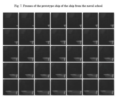
Fig. 6 illustrates a ship scale model used to perform the image reconstruction tests.

As observed in Fig. 8, the ship scale is reconstructed with all its details, results that constitute a big accomplishment because it is a low-cost method without contact that permits obtaining a 3D reconstruction of an isometric view of the object, under conditions of limited visibility.

Figs. 9 and 10 show the skeletonization process of the hull of a ship model shown in Fig. 6.

Conclusions

A methodology was presented for reconstruction of 3D images in murky waters or of poor visibility employing a high-resolution submarine camera and line laser. The method presents five steps: camera calibration, image capture, obtaining image patterns, triangulation and rendering. The methodology was applied to reconstruct a ship scale model, obtaining good results.

The methodology presents two important requirements for its effective application: constant speed and distance of the vehicle transporting the camera with respect to the object sought to capture and reconstruct its 3D image.

References

CACCIA, M. (2007). Vision-based ROV horizontal motion control: Near-seafloor experimental results. Control Engineering Practice, Vol. 15, pp. 703-714.

DEMA, M.A. (2006). 3D Reconstruction for Ship Hull Inspection. Master Thesis. Heriot Watt University. Scotland, UK.

DESERTSTAR, "Ship hull inspections with AquaMap", 2006, www.desertstar.com.

MONTALVO, M. “Técnicas de visión estereoscópica para determinar la estructura tridimensional de la escena”. Tesis de Maestría. Universidad Complutense de Madrid. 2010.

RAMÍREZ, J., VÁSQUEZ, R., GUTIÉRREZ, L., FLÓREZ, D. (2007). Mechanical/Naval Design of an Underwater Remotely Operated Vehicle (ROV) for Surveillance and Inspection of Port Facilities. Proceedings of IMECE2007 ASME 2007 International Mechanical Engineering Congress and Exposition, Seattle, Washington, USA.

REED, S., CORMACK, A., HAMILTON, K., TENA I., LANE, D. (2006). Automatic Ship Hull Inspection using Unmanned Underwater Vehicles. Proceedings of the 7th International Symposium on Technology and the Mine Problem. Monterey, USA. May, 2006.

VAGANAY, J., ELKINS, M., ESPOSITO, D., O’HALLORAN, W., HOVER, F., KOKKO, M. (2006A). Ship Hull Inspection with the HAUV: US Navy and NATO Demonstrations Results. IEEE/MTS Oceans’06, Boston MA, USA, Sept. 18-21, 2006.

VAGANAY, J., ELKINS, M., ESPOSITO, D., O’HALLORAN, W., HOVER, F., KOKKO, M. (2006B). Hovering Autonomous Underwater Vehicle for Ship Hull Inspection: Demonstration Results. Undersea Defense Technology Pacific (UDT Pacific ’06), San Diego CA, USA, Dec. 6-8, 2006.

ZAINAL, Z.B. (2007). Development of a Vision System for Ship Hull Inspection. Master Thesis. Universiti Sains Malaysia.