On the numerical prediction of the ship’s manoeuvring behaviour

Acerca de la predicción numérica del comportamiento de maniobra de la embarcación

Andrés Cura-Hochbaum¹

Abstract

A numerical procedure to predict the manoeuvrability of a ship based on Reynolds Averaged Navier Stokes simulations is described together with some recommended practices to obtain feasible results. The paper is dedicated to surface ships in unrestricted waters where usually only four degrees of freedom (DoF) are relevant. An example for a tanker shows the capability of the proposed method.

Key words: manoeuvring prediction, RANS, derivatives, virtual captive test.

Resumen

Se describe un procedimiento numérico para predecir la maniobrabilidad de un buque basado en simulaciones Reynolds promediadas de Navier Stokes, así como algunas prácticas recomendadas para obtener resultados factibles. Este documento está dedicado a embarcaciones de superficie en aguas sin restricciones donde usualmente sólo cuatro grados de libertad son relevantes. Un ejemplo para un buque cisterna muestra la capacidad del método propuesto.

Palabras claves: predicción de maniobrabilidad, RANS, derivados, prueba de cautivo virtual.

Date Received: January 23th, 2011 - Fecha de recepción: 23 de Enero de 2011
Date Accepted: February 17th, 2011 - Fecha de aceptación: 17 de Febrero de 2011

________________________

¹ Technical University Berlin, Department Dynamics of Maritime Systems. Berlín. Germany. e-mail: cura@tu-berlin.de

............................................................................................................................................................

Introduction

RANS tools, i.e., numerical methods for solving the Reynolds Averaged Navier Stokes equations for viscous turbulent flows, can be applied to predict the manoeuvring behaviour of a vessel. This is achieved either directly, by using the considered RANS code for calculating the hydrodynamic forces and moments acting on the hull in every new time step of the simulated rudder manoeuvre, or by using it to calculate the time histories of these forces and moments during selected forced motions. The latter results can be used to determine the manoeuvring derivatives of a mathematical model for manoeuvring prediction.

This second procedure is described in this paper from the practical point of view, together with recommended practices to obtain feasible manoeuvring prediction results. The numerical techniques used to discretise and solve the partial differential equations involved, e.g., finite difference method or finite volume method, to model the flow turbulence and to generate grids, have been described in many publications (Ferziger and Peric 2002, Wilcox 1993, Thompson et al., 1985). This paper is dedicated to surface ships in unrestricted waters, where usually only four degrees of freedom (surge, sway, yaw, roll) are relevant for manoeuvring. In the example shown here for a very large crude carrier, however, the roll motion has no significant effect.

Manoeuvring Simulation

To predict a manoeuvre, the rigid motion equations of the ship in 3-DoF, 4-DoF, or even in 6-DoF are numerically integrated in time with a proper discretisation scheme, e.g., Euler implicit, Runge-Kutta, etc. In most applications, provided large accelerations are not expected, the first-order Euler explicit scheme can also be used. The motion parameters considered should be properly defined by means of an earth-fixed or “inertial” coordinate system, a ship-fixed coordinate system and/or with help of an intermediate or “hybrid” coordinate system to uniquely define angles and translations. The singularity typically (gimbal lock, for cos θ=0) occurring when using Euler angles is not relevant for a surface ship.

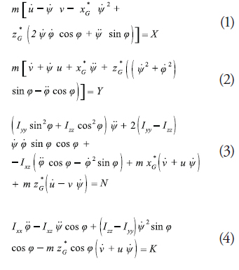
An example of motion equations in four degrees of freedom (4 DoF) for a free sailing (rigid) ship or model written in a hybrid coordinate system, which follows the ship motions excepting roll, reads:

The surge and sway velocities u and v are the components of the velocity of the chosen ship origin O in the horizontal longitudinal and transversal directions x and y of the hybrid coordinate system, respectively. The Euler angles and are the rotations around the x- and y-axes, respectively and describe the ship’s roll and yaw motions. The dots in the equations above denote time derivatives. m is the mass of the ship or model and x_G* and z_G* are the coordinates of the centre of gravity, G, in the ship’s fixed system. It is assumed that y_G* =0. I_xx, I_yy , I_zz are the moments of inertia about the ship’s fixed axes through the origin O and I_xz is the product of inertia. It is assumed that I_xy* 0 and I_yz* 0 because of symmetry. X and Y (longitudinal and side forces) are the components in the hybrid system of the external force acting on the ship. K and N (roll and yaw moment) are the components in the hybrid system of the moment of the external forces. Given that heave and pitch motions are neglected, the state of movement of the ship is defined by the position of O (earth-fixed coordinates), its velocity vector (u, v, 0), the Euler angles , , and the angular velocity vector . The time history of these variables can be obtained by integrating equations (1) to (4) numerically over time. For this purpose, the forces and moments on their right hand sides are needed.

Rudder manoeuvres, like zigzag tests and turning circle tests, can be simulated directly by solving together equations (1) to (4) for the ship and the RANS equations for the fluid to calculate the forces and moments in every new time step. The rudder(s) is (are) turned according to the desired manoeuvre during the simulation. This kind of manoeuvring simulation is extremely timeconsuming but, since there is no mathematical model for the hydrodynamic forces involved, in principle it is easier than by means of manoeuvring derivatives. It will represent the best approach once comprehensively validated. Some publications already show the potential of this procedure (Carrica et al., 2008).

Rudder manoeuvres are traditionally simulated by using a mathematical model to calculate the hydrodynamic forces and X, Y, K, and N moments in every new time step of the time marching procedure used when solving the motion equations of the ship. An approach based on Abkowitz-type coefficients reads, e.g., for the non-dimensional side force:

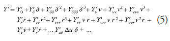
The force has been written as a function of the rudder angle, δ, expressed in radians; the nondimensional surge and sway velocities Δu=(u-U₀) /U₀ and v/U₀, where U₀ is the initial speed of the ship and the non-dimensional yaw rate r = L_pp /U₀, where L_pp is the ship length. The approach includes terms up to the third order and also mixed or coupled terms, accounting for interactions, but many other terms could be added. The sub-index u represents Δu. Dots denote time derivatives. Thus , for instance, represents the hydrodynamic mass for transverse motion. Forces are made nondimensional with and moments with , ρ being the water density. All magnitudes in Equation (5) have been made non-dimensional with proper combinations and powers of and L_pp. Except for the coefficients, primes have been omitted for simplicity.

The coefficients are usually determined by means of captive model tests performed with a Planar Motion Mechanism (PMM) or a Computarized Planar Motion Carriage (CPMC). Once the coefficients have been determined for a specific ship it is very simple to predict all desired manoeuvres.

Manoeuvring Simulation

Due to the enormous computational effort required for the direct simulation of manoeuvres, another CFD (DEFINE FIRST) strategy has gained popularity instead. It consists in simulating usual PMM or CPMC tests numerically, solving the RANS equations around the ship or ship model when performing prescribed motions. Compared to direct manoeuvring simulations, this prediction procedure has the same advantages and disadvantages as between free and captive model tests. From the computational point of view, however, it is definitively more robust and less time consuming.

The strategy fully resembles the classical, wellaccepted PMM tests followed by the determination of derivatives and seems already practicable for commercial applications. Nevertheless, a mathematical model (i.e, a set of coefficients of Abkowitz type or coefficients of formulae for diverse forces of a modular simulation method) is involved, introducing a further source of uncertainty into the prediction.

Motion equations are not solved in this instance. Selected motions, i.e., harmonic pure sway, pure yaw, etc, are imposed; there are different ways to impose the motions. In order to resemble CPMC tests or to reproduce measured motions during free-model tests, it can be advantageous to read a file containing the time histories for the motion parameters.

Note that when disregarding that the ship motion is given, it would be best to let the ship or free model to sink and trim during the RANS simulation. However, contrary to direct manoeuvring simulations with RANS where the motions are predicted anyway and merely two more DoF should be considered to include sinkage and trim, this is less straightforward now and leads to a combination of given and predicted motions.

The analysis of the predicted time histories of the longitudinal and transverse forces X, Y, and the roll and yaw moments K, N is the same as when performing PMM or CPMC model tests. Moreover, since no artifcial time lag between predicted forces and prescribed motions arise and no inertial forces have to be subtracted (no filters, no swinging masses), the analysis is easier than performing model tests.

Similar to when performing model tests, there are different ways of determining the manoeuvring derivatives and the “virtual” test program has to be decided according to this and to the mathematical model used (e.g. the derivatives to be determined). The first step of any numerical investigation for manoeuvring consists in analysing the case considered and making decisions like limiting the calculations to double body flow or taking the free water surface into account, considering the free sinkage and trim or not, performing the simulations for the ship model or for the full-scale ship. This is followed by the proper choice of a turbulence model, discretisation schemes, grid and time resolution, and the choice of the boundary conditions at the borders of the grid.

In addition, several parameters of the code employed usually have to be chosen as well; for instance: the number of (outer) iterations within each time step, the number of (inner) iterations within an outer iteration, values for diverse underrelaxation factors, among others. Depending on the code, other settings could also be required and strongly influence the result of the computations. For these reasons, experience in viscous flow computations and insight on the RANS code to be used are prerequisites for successful CFD-based manoeuvring prediction.

General Considerations

In principle, RANS simulations can be performed for the full-scale ship, avoiding any scale effect. In practice, however, most simulations are performed for the model rather than for the full-scale ship because computations for Reynolds numbers in the order of 109 are yet to be fully validated and yield much more numerical difficulties than for Reynolds numbers at model scale, being two orders of magnitude smaller. In addition, prediction results for the model can be judged as a whole by comparing them with the results of a few selected free-model tests.

The Navier-Stokes (NS) equations and the continuity equation describe the conservation of momentum and mass in a viscous turbulent incompressible flow and are best suitable to describe the flow around a ship. To work with mean values of all flow variables (e.g. velocities, pressure) instead of instantaneous values, the RANS equations are obtained by averaging the NS equations. This averaging can be seen as time averaging in case of a steady mean flow, but has to be understood as ensemble averaging in case of an unsteady mean flow (Wilcox 1993, Cebeci et al., 2005). As a result of the averaging, the RANS equations contain some new unknown terms representing the effect of the turbulence on the flow. In order to solve the set of conservation equations, these terms are approximated by a turbulence model. The reason for doing so is that if not, the required space and time resolution for directly solving the NS equations would be impracticable (probably still in the next decades) for a turbulent ship flow.

Any turbulence model used by usual RANS applications can also be used for manoeuvring tasks. The most popular models are the k-ε and k-ω models (Launder and Spalding 1974, Wilcox 1993) and several variants with and without using wall functions, which allow a significantly coarser resolution of near-wall regions. When looking for accurate prediction of complex flow phenomena, however, e.g. detailed flow separation, more sophisticated turbulence models like Reynolds Stress Models (RSM) could be a better choice (Wilcox 1993). But, such models are less validated and often less robust and more time-consuming than the classical two-equation models mentioned above.

The experience from published results and workshops shows that the dependence of side force and yaw moment on the turbulent model, i.e., of those forces which are most significant for manoeuvring, is less significant than expected. The reason is that these hydrodynamic forces are certainly viscosity dependent but firstly dominated by pressure. In fact, satisfactory results can be achieved even by using wall functions as they do not deteriorate the quality of the predictions to the same extent than when predicting resistance.

Disregarding cases where RANS tools are used for predicting forces on the bare hull only, e.g. to determine coefficients for hull forces in a modular mathematical model, the appendages have to be considered for manoeuvring tasks. Inclusion of rudders and even bilge keels has become usual in RANS applications. This complicates the grid generation and probably also some flow aspect, which can lead to increased convergence difficulties, but does not really represent a problem.

The main issue is how to treat the propeller(s), crucial for simulating the rudder inflow correctly when rudders are placed behind propellers. Taking the real geometry of the propeller into account and considering the rotating propeller during the RANS simulation is possible but extremely time consuming. Thus, body forces, which are added to the right hand sides of the RANS equations, are frequently used to approximate the effect of the propeller on the flow. These forces are distributed over the grid region corresponding to the spatial position of the propeller and are calculated so that they yield the propeller thrust and moment.

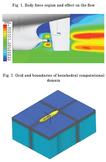
Body force models, mostly based on potential flow codes like vortex-lattice or panel methods, are often used to approximate the propeller effect including slip stream and swirl, which may also influence aspects of the flow like rudder stall angle, risk of cavitation, etc. The body force distribution inside the propeller region may be calculated in every new time step or in some larger time intervals, based on the current propeller inflow obtained during the RANS simulation and on the propeller rpm. This can be done either interactively, running the used potential code each time again, or determining the forces in grid cells within the propeller region from a data base calculated beforehand for the considered propeller. Fig. 1 shows the cylindrical body force region (rectangle) and the effect of the body forces on the axial velocity in the longitudinal central plane.

The choice of the propulsion point, corresponding to the full scale or to the model scale, should be decided by following similar criteria as for model tests. A way of determining the correct propeller rpm before starting the manoeuvre simulation is to calculate the flow for the steady straight ahead motion of the ship at the given approach speed for different rpm’s and to determine the one which makes the total longitudinal force equal to the desired value (e.g. zero or estimated frictional deduction). A proper strategy for the propeller rpm dur-ing the manoeuvre, resembling the real behaviour in full scale where the rpm often varies depending on torque, can also be implemented.

Commercial grid generators are widespread, but open source software is also gaining in popularity recently. Block-structured grids, often including non-matching interfaces, and unstructured grids with several million cells have become usual for manoeuvring tasks. Contrary to many CFD applications for ship resistance or propulsion, the nature of the problem now requires a grid covering the surroundings at both sides of the ship.

Not only for turning the propeller but also to deflect the rudder within direct manoeuvring simulations, a RANS code with sliding grid or overlapping grid capability is needed (Carrica et al.,). In the later case, a considerable amount of computational effort is required to transfer flow information from one grid part to the other. Otherwise and whenever possible, the grid is kept unchanged during the computation to avoid deteriorating its quality, which directly influences the convergence behaviour and the quality of the results. Nevertheless, this is obviously not possible in many cases of interest, for example when considering squat in shallow water or approaching a quay. In such cases, a suitable grid deformation technique can be an alternative to overlapping grids.

The grid can be generated in several ways and many different grid topologies can be chosen. The outer boundaries of the grid mostly consist of planes delimiting a box (hexahedron) surrounding the ship. Fig. 2 shows a typical configuration for a manoeuvring application for a double-body in deep water.

The grid has to cover the interesting flow domain so that non-physical boundaries (see below) are far from the region of interest, i.e., ship vicinity. Typical dimensions of a grid are 3-5 ship lengths in longitudinal direction, 2-3 in transverse direction and one length in vertical direction for deep water. The near-wall region has to be meshed so that the requirements of the used turbulence model are fulfilled (Wilcox 1993, Menter 1994). In any case, a certain number of grid points (say 20) within the boundary layer have to be placed. For the reasons mentioned above regarding the influence of viscosity on side force and yaw moment, wall functions are often used for manoeuvring cases.

If the flow computation is made in a ship-fixed coordinate frame, i.e., if the conservation of momentum is stated in terms of its components in a ship-fixed coordinate system, inertial body forces, e.g. centrifugal and Coriolis forces, have to be added to the RANS equations (Cura and Vogt 2002). These forces are usually treated explicitly during the computation and could affect the stability and convergence of the computation if they are considerably larger than the hydrodynamic forces themselves. On the other hand, if the flow computation is made in an earth-fixed or inertial coordinate frame, no inertial forces have to be added but cell boundary velocities will have to be considered to calculate the correct mass and momentum fluxes through the cell sides; see for instance Ferziger and Peric 2002. Both proce-dures are mathematically equivalent. The numerical advantages of one or the other procedure seem not significant for typical manoeuvring applications.

The boundary conditions (BC) are crucial for the accuracy of the numerical solution. Setting nonphysical boundary conditions such as undisturbed flow (Dirichlet) or zero-gradient (Neumann) too close to the ship will affect the results. The way BC are imposed within the numerical technique may change from code to code, but does not differ for manoeuvring tasks from other tasks. However, during manoeuvring simulations there are often no longer unambiguous inlet or outlet borders of the computational domain but mixed forms. Further, in unsteady flow cases, the BC may have to be updated during the course of the simulation according to the instantaneous ship motion.

At an “inlet” border for instance, far in front of the ship (e.g. 1 Lpp) the absolute velocity is zero (in absence of current and waves). Within a ship-fixed frame, however, inlet velocities are relative velocities and, therefore, of equal magnitude but opposite sign than the velocity resulting in the considered point of the boundary from the translation (ship velocities u and v) and rotation (yaw rate r) of the ship-fixed coordinate system, i.e., u inlet = – ( u –y r ) v inlet = – ( v + x r )

A pressure BC, either zero pressure for doublebody flow or undisturbed hydrostatic pressure distribution for free surface flow, has proven be advantageous for the “outlet” border far behind the ship (e.g. 2-4 Lpp).

At the sides of the computational domain, e.g. placed 1-2 Lpp away from the ship, the velocities may also be given, but these borders could also be treated as inlet and outlet boundaries, for instance in case of a steady oblique towing motion at large drift angle.

At rigid walls like the hull, a “no slip” BC is mostly set, ensuring that the fluid particles have the same velocity as the wall. Sometimes, however, it is convenient to consider a wall without any friction, a “free slip” wall, for instance to delimit the computational domain. Note that, if planar, such walls behave similarly to symmetry planes.

The bottom of the computational domain can be seen as a free slip wall placed far below the ship for deep water (e.g. one Lpp). The same can be chosen for the top border of the considered hexahedral domain, placed at the waterline in case of doublebody flow or at some distance (e.g. 0, 1 – 0, 3 Lpp) above the waterline in case of a free-surface flow.

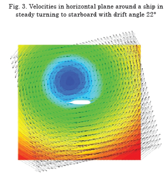
Note that during manoeuvres often no real inlet and outlet boundaries exist and a border of the computational domain may change its character during the simulation. For these reasons, some adapted “mixed” BC taking this feature into account have proven advantageous. Hereby, the velocities are given if the flux is directed into the domain only and they are let free otherwise. This has been done at the left, upper and lower lateral borders in the example of Fig.3, while undisturbed pressure was assumed at the right border. The calculated velocity field differs from the undisturbed field in the close vicinity of the ship only.

Computations can be performed by taking the water free surface into account or not. The latter approach is reasonable for a slow ship in deep water and requires significantly less computational effort (e.g. factor 10 in a steady case). Nevertheless, even at low Froude numbers, the underwater shape and, thus, the forces could change significantly if the sinkage and trim of the vessel vary at large drift angle or yaw rate. A way to take such changes into account would be by including the free surface and using a 6 DoF motion model (see below) letting the ship free to sink and trim during the simulation.

Including the water free surface, however, even having become more standard in the last years, leads not only to more computational time but also to increased numerical difficulties. In particular, reflection of the waves generated by the ship on non-physical or open boundaries (outlet) should be avoided. Among other techniques to avoid such reflections, a strong coarsening of the grid towards the outlet has proven efficient in damping the outgoing waves, preventing reflections in a rather rude manner. This procedure would not be applicable if the boundary considered changes its type (e.g. from outlet to inlet) in the course of the simulated manoeuvre.

Example

The technique outlined above is applied here to predict the manoeuvrability of a Very Large Crude Carrier (VLCC), namely the tanker KVLCC1, used as a benchmark test in SIMMAN’08. Due to the low Froude number of the considered tanker and because negligible heel angles are expected during its manoeuvres, all RANS simulations were performed without taking the water free surface into account.

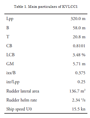
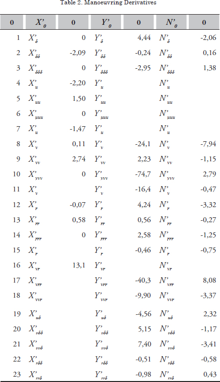
An in-house RANS code was used to calculate the flow around the tanker at several static conditions and during virtual pure surge, pure sway, pure yaw, and combined sway-yaw tests to obtain a rather simple set of hydrodynamic Abkowitz-type coefficients (Table 2).

All dynamic tests were simulated by using the same multi-block structured grid with about one million cells with (some) non-matching block interfaces. The semi-balanced horn rudder, embedded in an individual grid box, is not deflected during these simulations. For static cases with deflected rudder and constant drift angle and/or yaw rate only this grid box is replaced by another according to the rudder angle considered.

The grid dependency of the results has to be checked at least by means of selected calculations on different grids. In the present case, the values of all forces and moments acting on the ship obtained on coarse, medium, and fine grids behaved consistently and differed by less than 10% from each other. Although this check cannot replace a real Uncertainty Analysis (UA) it may be a good compromise in practise.

The computations are performed on a ship-fixed grid using a Cartesian non-inertial coordinate system. The standard two equation k-ω turbulence model with wall functions is used. During dynamic tests, the motions are imposed through the boundary conditions and corresponding inertial forces added to the RANS equations, see Cura and Vogt (2002).

Currently, the needed CPU time to simulate dynamic test amounts is still several days per period on a single processor of a normal PC, but it can be much less if a parallel code is run on a cluster with hundreds of processors. The static tests usually take some few hours depending on grid resolution.

Vortex lattice data for the propeller of a typical tanker was used in the present case. The rate of revolutions was set so that the resulting thrust balanced the resistance computed during a steady straight ahead motion of the model (model self propulsion point). This rate was kept constant throughout the computations. Fig. 5 shows the velocity distribution just behind the propeller plane during a simulated combined sway-yaw test at a certain time when the ship is turning to starboard. The white circle indicates the body force region.

In order to obtain all manoeuvring derivatives, except those depending on the rudder angle and surge velocity, five dynamic tests with large velocity amplitudes and a common non-dimensional period T ’ = T U0 / Lpp of 3.369 (20 seconds in model scale) are simulated. Similar to real tests, the non-dimensional amplitudes of the harmonic motions should be chosen so that they cover the expected range of the motion parameters during the manoeuvres. In the present example, the amplitudes were: Δu’ = Δu/ U0 = 0.10 for pure surge, v’ = v / U0 = 0.35 for pure sway, r’ = r Lpp / U₀ = 0.70 for pure yaw and -0.35, 0.20 and -0.20, 0.40 for two sway-yaw tests, respectively.

The simulations were carried out for the tanker model (scale 1:45.7) at a speed of 1.179 m/s, instead of for the full scale. The time step chosen for the RANS simulation corresponded to 1/2500 of the motion period in all cases.

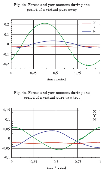
The hydrodynamic forces and moments acting on the ship are obtained by integrating the pressure and shear stresses on the hull and appendages. The predicted time histories over one period of the simulated pure sway and pure yaw tests can be seen in Fig. 4. The longitudinal force X’, side force Y’ and yaw moment N’ have been made non-dimensional with water density, ship speed, length, and draught. Rudder angle, depending manoeuvring derivatives, can be determined by computing rudder angle tests at several drift angles and yaw rates resulting in a total of 42 cases.

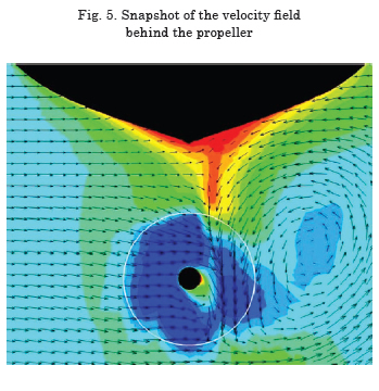
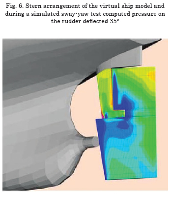
Fig. 6 shows the stern arrangement of the virtual model of KVLCC1 with the rudder deflected 35° to starboard. The pressure field on the rudder computed for steady straight ahead motion is influenced by the effect of the propeller, rotating to the right over the top. Negative pressure regions are depicted in blue, while positive pressure regions are in red.

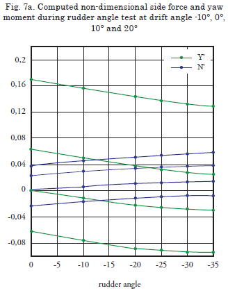
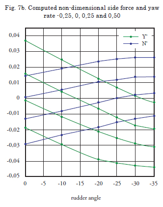
The computed non-dimensional side force and yaw moment acting on the hull for all static cases are summarised in Fig. 7 for oblique towing and steady turning conditions, respectively.

The time histories of the forces obtained from the RANS simulations for the five dynamic tests described above are used to determine the coefficients of the mathematical model in the same way as if PMM tests would have been done. This yields the coefficients in rows 4-18 of Table 2.

Regression analysis of the data obtained from static cases with deflected rudder yields the coefficients depending on the rudder angle written in rows 1-3 and 19-23 in Table 2.

The hydrodynamic coefficients shown in Table 2 have been made non-dimensional with water density, ship speed and length and multiplied by 1000, and are used to simulate standard rudder manoeuvres according to IMO (2002). For this purpose, the motion equations of the ship in four degrees of freedom (4 DOF) were used. However, the dependency of the non-dimensional magnitudes X’, Y’, N’, and roll moment K’ (not shown) on heel angle and roll rate was neglected because no significant roll motion was expected for the considered tanker. The sub-indices u, v, r and δ denote the surge, sway, and yaw velocities and the rudder angle, respectively.

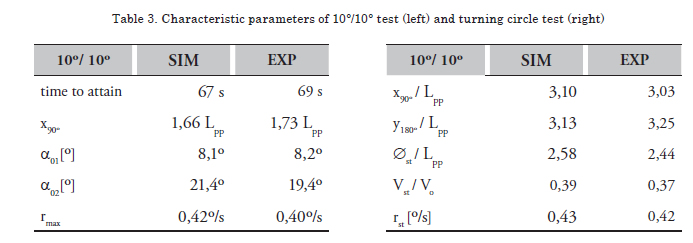
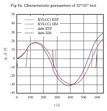
The main results of the simulated 10°/10° zigzag test starting at starboard are compared with experimental results in Fig. 8, which shows on the left side the heading angle, ψ, and the rudder angle, δ, versus time. The 2^nd overshoot angle predicted for KVLCC1 is slightly larger than that measured and the overall agreement deteriorates with increasing time. Nonetheless, the characteristic parameters used to judge yaw checking and initial turning ability are predicted well, Table 3.

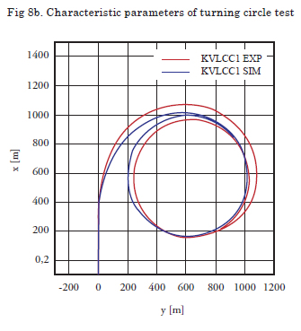
Any other rudder manoeuvre of interest can be predicted, as well. For instance, the result of a simulated turning circle to starboard with a rudder angle of 35° is compared with a free-model test in Fig. 8b. The main parameters of the turning circle tests are compared with experiments in Table 3 showing good agreement. Note that the tanker fulfils the IMO recommendations with margin.

A detailed comparison of all results obtained with this method and with several other methods for manoeuvring prediction from other authors with experimental data is documented in the proceedings from the SIMMAN 2008 Workshop (Stern and Agdrup 2009). As can be seen, there the results of the present pure CFD-based method belong to the best results in the case considered.

References

ABKOWITZ, M.A., (1964), "Lectures on Ship Hydrodynamics - Steering and Manoeuvrability", HyA Report HY-5, Copenhagen.

CARRICA, P.M., ISMAIL, F., HYMAN, M., BHUSHAN, S., AND STERN, F. (2008), "Turn and zigzag manoeuvres of a surface combatant using a URANS approach with dynamic overset grids", SIMMAN 2008, Copenhagen Cura Hochbaum, A. and Vogt, M. (2002), "Towards the Simulation of Seakeeping and Manoeuvring based on the Computation of the Free Surface Viscous Ship Flow", 24th ONR Symposium on Naval Hydrodynamics, Fukuoka.

CURA HOCHBAUM, A. (2006), "Virtual PMM Tests for Manoeuvring Prediction", 26th ONR Symposium on Naval Hydrodynamics, Rome.

CURA HOCHBAUM, A., VOGT, M., GATCHELL, S. (2008), "Manoeuvring prediction for two tankers based on RANS calculations", SIMMAN 2008, Copenhagen.

IMO, International Maritime Organization, (2002), Resolution MSC.137(76), "Standards for Ship Manoeuvrability", London.

FERZIGER, J.H., PERIC, M. (2002), "Computational Methods for Fluid Dynamics", Springer.

HIRT, C.W., AND NICHOLS, B.D. (1981), "Volume of Fluid (VOF) Method for the Dynamics of free Boundaries", J. of Comp. Physics, Vol.39.

LAUNDER, B.E., AND SPALDING, D.B. (1974), "The numerical computation of turbulent flows", Comput. Meth. in Appl. Mech. Eng. Vol.3.

MENTER, F.R. (1994), "Two-Equation Eddy- Viscosity Turbulence Models for Engineering Applications", AIAA Journal, Vol.32, No.8.

OSHER, S., AND SETHIAN, J.A. (1988), "Fronts Propagating with Curvature-Dependent Speed: Algorithms Based on Hamilton-Jacobi Formulations", J. of Comp. Physics, Vol.79.

STERN, F. AND AGDRUP, K. (editors) (2009), "Proceedings of the Workshop on Verification and Validation of Ship Manoeuvring Simulation Methods SIMMAN 2008", FORCE Technology, Lyngby, Denmark

THOMPSON, J.F., WARSI, Z.U.A., MASTIN, C.W. (1985), "Numerical Grid Generation: Foundations and Applications", North Holland, New York Wilcox, D.C. (1993), "Turbulence Modeling for CFD", DCW Industries, La Cañada, California