Aid in the Design of Antenna Arrays with Electronic Phase Steering using Matlab®
Ayuda al diseño de arrays de antenas con direccionamiento electrónico de haz empleando MATLAB®.
Francisco José Gil Navia1
Abstract
Antenna arrays have been used since the 1950s in multiple applications; however, it was not until recent years that, given progress in digital technologies, this application has become the fastest and most varied development in the radar world. The main motivation for their development is that they permit electronic phase steering that implies extreme phase agility, while also being tolerant to failure because of the amount of elements that comprise them. They also permit the reduction of side lobes by controlling the amplitude of each element.
Because it is a currently applied technology, but with many aspects under development, it is necessary to enter this field and generate the required tools including those for computer assisted prototyping. Because of the aforementioned, this work sought to use Matlab® to create virtual prototypes of arrays that permit visualizing an approach to their real behavior stemming from certain parameters.
Key words: Antenna arrays, electronic phase steering, MATLAB.
Resumen
Los arrays de antenas han sido empleados desde los años cincuenta en múltiples aplicaciones, sin embargo no ha sido hasta años recientes que, gracias a los adelantos en tecnologías digitales, se ha logrado convertir esta aplicación en la de más rápido y variado desarrollo dentro del mundo radar. La principal motivación para su desarrollo es que permiten el direccionamiento electrónico de haz que implica una agilidad de haz extrema, además son muy tolerantes a fallos por la cantidad de elementos que los componen. También permiten la reducción de lóbulos laterales por medio del control de la amplitud de cada elemento.
Por ser una tecnología aplicada actualmente pero con muchos aspectos en desarrollo se hace necesario adentrarse en este campo y generar las herramientas necesarias incluyendo aquellas de prototipado mediante computador. Por lo anterior en este trabajo se pretende emplear Matlab® para crear prototipos virtuales de arrays que permitiría visualizar una aproximación al comportamiento real de los mismos a partir de ciertos parámetros.
Palabras claves: Arrays de antenas, Direccionamiento electrónico de haz, MATLAB.
Date received: September 10th, 2010 - Fecha de recepción: 10 de septiembre de 2010
Date Accepted: November 1st, 2010 - Fecha de aceptación: 1 de Noviembre de 2010
________________________
1Departamento de Armas y Electrónica de la Armada Nacional, Fuerza Naval de Caribe, Base Naval 1. Colombia.
E-mail: francisco.gil@armada.mil.co
............................................................................................................................................................
General considerations on Arrays with Electronic Phase Steering
Antenna arrays with electronic phase steering are antenna groups arranged in space in such a way that they permit obtaining a desired radiation pattern. In practical applications, the elements tend to be in linear or plane arrangement, in regular polygonal or circular form; additionally, these can also form crosses or diamond shapes amongst themselves. The spacing between elements is normally uniform. Also, active and passive elements are combined [2].
Types of Electronically Guided Arrays
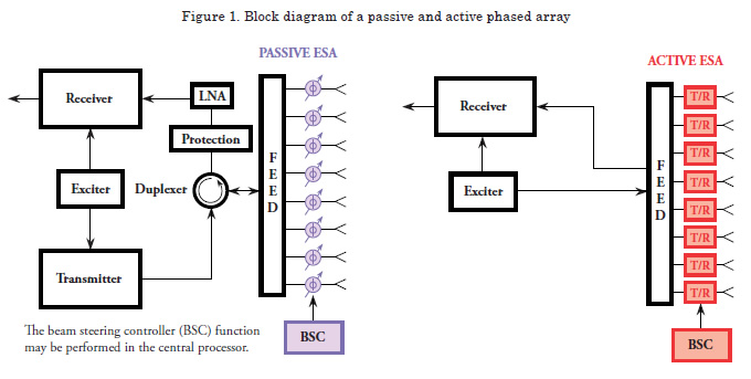
There are two basic types, passive and active.
Passive Arrays
Consists of a sole transmitter whose signal is distributed to the different elements with the signal phase being modified in each element via a phase shifter [3].
Active Arrays
Consist of individual transmission and reception modules. Each module has a phase shifter, a high-power amplifier (HPA), a duplexer, which permits communicating between signal transmission and reception, a protection system that keeps transmission residue from filtering into the reception, and a low-noise amplifier for the receptor.
In both cases, the phase shifters are controlled via a beam steering controller (BSC).
Advantages of Arrays with Electronic Phase Steering
Extreme phase agility (in the order of milliseconds) permits performing multiple simultaneous tasks like monitoring several simultaneous targets or monitoring and searching at the same time. This is accomplished through spatial, temporal, or spectral multiplexing, or all of them [4].
Besides, it saves energy and the complex systems that involve the antena addressing using servomotors. It also present little or no aperture blockage.
Another important advantage is that they permit accomplishing lower RCS on the platform on which they are mounted [2].
Additional advantages of Active Arrays
Because the transmitter high-power amplifiers and the receptor low-noise amplifiers are near the antenna, la signal-noise ratio will always be lower.
Permit controlling the lighting function, which permits reduction of side lobes.
Permit the generation of different phases pointing in different directions to different frequencies through the partition of the array into sub-arrays [2].
Limitations of Arrays With Electronic Phase Steering
The greater the pointing angle, with respect to the center, the lower the gain in the main phase and greater level of side lobes. As a general rule, the maximum pointing angle is ±60°.
The high cost, each transmission receptor module costs around US$2000. An array can have between 1000 and 2000 modules, which may mean a cost of up to 4-million US$ [2].
Electric Field of an Antenna Array
An array is formed by two or more radiators. These radiators are called elements. These elements may be of any type: dipoles, dishes, slots etc.
The electric field formed by array of “n” elements, in each “i” far field point with (Θi,) direction, is the sum of the individual electric fields of each element in that point.
![]()
In the far field, it may be considered that the lines between each element and the point are parallel and, hence, the θ and φ angles are equal.
Also, the phase with which each signal reaches the point in space will be different. This can be found by calculating the difference of the distance travelled by the signal transmitted by each element to reach each point, obtaining the point product between the “q” propagation direction and the “d” distance vector for each emitter with respect to the point of reference. [6]
![]()
Assuming that the electromagnetic waves propagate in cosine form and that the phase of a signal originating at the point of reference reaches the far field with zero phase, it is possible to determine the ![]() phase with which all the signals arrive from their very wavelengths and the
phase with which all the signals arrive from their very wavelengths and the ![]() distance.
distance.
If we now incorporate the “In” illumination function represented by the signal width for each of the elements, we have the magnitude of the electric field in each direction (θ,φ).
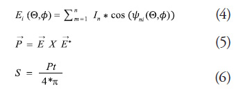
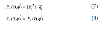
Power and Power Density
From equation (4), and using equations (5) and (6), we calculate the magnitude of the power density in each “i” point – knowing that the direction is the same as that of the propagation vector, hence.
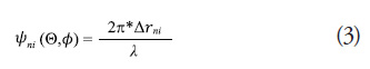
Electronic Phase Steering
Electronic phase steering1 is accomplished by changing the initial phase with which the signal is transmitted in each element. This gap is done by successively delaying the signal between the adjacent elements. The ![]() gap between the adjacent elements is proportional to the “d” distance between the elements. This means that the electric field generated by the array in the different directions would be given by.
gap between the adjacent elements is proportional to the “d” distance between the elements. This means that the electric field generated by the array in the different directions would be given by.
![]()
Where ![]() Θ is the phase with which the signal arrives without delaying it, to the point in the far field.
Θ is the phase with which the signal arrives without delaying it, to the point in the far field.
If we wish to vary the pointing angle of the main phase in a “β” angle, a delay must be applied to the signal that produces a phase variation according to the following relation:
Where ![]() is the signal wavelength.
is the signal wavelength.
Granularity of the Phase Shifters
Given that the phase variation in the different elements of the array is done with phase shifter elements that operate discretely through a binary control, the capacity of pointing the phase in a determined direction without degrading the radiation pattern (dimensions of main lobe and height of side lobes) depend on the amount of bits permitted by the phase shifter and the number of elements of the array. The minimum leap in angular phase units that each phase shifter can perform in function of the amount of bits available is denominated granularity and is given by equation (11) [4].
Measurable Parameters
Width of the Main Lobe
Obtained by measuring the angle formed from the origin by the points of media power of the radiation pattern.
Level of Side Lobes
In practice, there is commitment among the level of the side lobes, the width of the main lobe, and the directivity. The most accepted means to assess the level of side lobes is by comparing the highest of these, on the logarithmic scale, with the main lobe.
Aspects not considered
For effects of this work, we will not bear in mind the mutual impedance between elements and polarization.
The Program
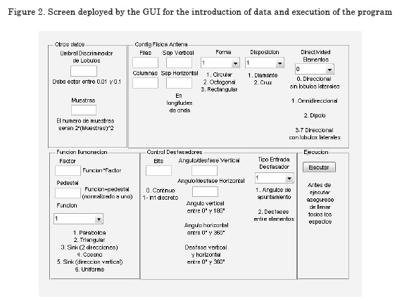
The program was developed in Matlab®, including the graphic user interface (GUI) through which the data are introduced and from which it is executed.
The software has a friendly interface that allow the data ingress to it's performance. The data to be introduced, shown in Figure 2, are:
Other data
For effects of this work, we will not bear in mind the mutual impedance between elements and polarization.
Number of samples per pi radians arc: The number of samples in the whole sphere is 2*S2.
Lobe discriminating threshold: This control permits adjusting a threshold that will allow adequate discrimination of the lobes for each particular case. This is implemented because in some cases the lowest level where the lobes are differentiated are too high and, hence, the program can assume that two different lobes are only one, producing errors. The most recommended value is 0.005.
Physical Configuration of the Antenna
Lighting Function
The function can be selected from the following: (1) parabolic, (2) triangular, (3) sink, (4) cosine, or (5) uniform. In addition, it may be defined to what power the function selected is raised except for the uniform function that can only be raised to the first power.
The pedestal of the lighting function permits adding a reference value for the function greater than zero.
Phase Shifters
These permit selecting if the phase shifter is analogous (continuous) or digital (discrete); it also permits data input in two ways. In the first, the phase pointing angle is input in spherical coordinates (θ,φ). In the second form, the degrees of gap between consecutive elements are input.
Execution
This triggers the execution of the whole program. Be sure to have input all the data before executing the program; on the contrary, error will be produced.
Graphics
The results are deployed through graphics that can be manipulated by users.
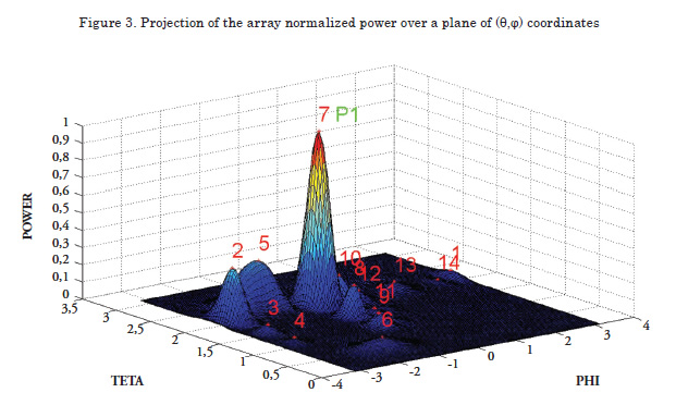
Power in spherical coordinates (Θ,Φ) projected on a plane
This graphic permits better visualizing the peak powers for each of the lobes and permits more easily locating the spherical coordinates of said points. It has the disadvantage of distorting the radiation pattern, given that a three-dimensional volumetric form is being represented on a plane.
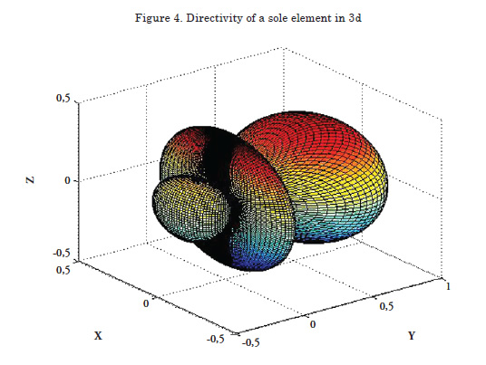
Directivity of a sole element
This graphic permits visualizing the radiation pattern of a sole element.
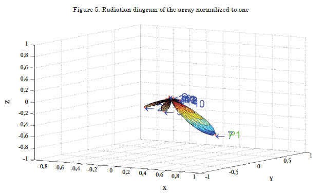
Radiation pattern of the Array
The radiation pattern permits visualizing the location of each of the lobes in three dimensions, numbering them in such a manner that they can be compared with the measurements. Additionally, the main lobe is distinguished with the green letter “P”, followed by a number that indicates, in case of more than one main lobe, the corresponding lobe.
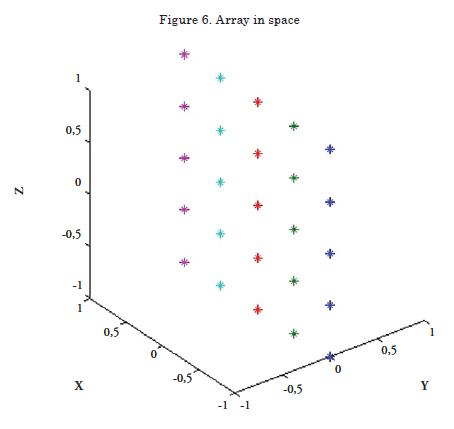
Array in space
It permits visualizing the shape, number of elements, and their disposition in space.
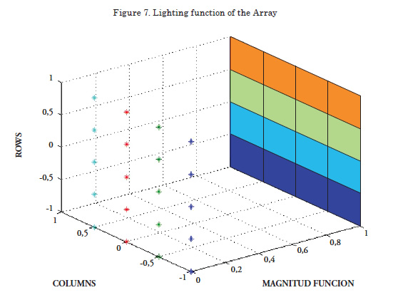
Lighting Function
This permits graphically visualizing the lighting function of the array. The surface of colors represents the values of the lighting function for each element.
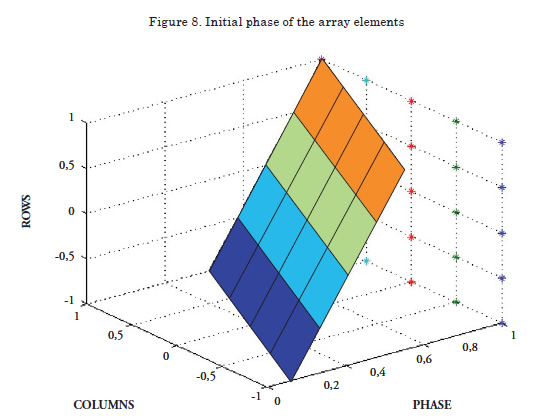
Initial Phase of the elements of the Array
It permits seeing graphically the initial phase of the array elements. The values of the initial phase form a surface of colors whose values are interpolated on the coordinate called “phase”.
Results
The linear antenna is the base for the design of planar arrays, given that they represent the simplicity of performing analysis in two dimensions rather than three. For this case, we take a linear antenna of three omnidirectional elements; each separated from the other by half a wavelength, with a constant lighting function in all and a zero pointing angle.
Width of the Main Lobe in function of the pointing angle
To test the functioning of the program, two references are taken. The first is the approach made by M. Skollnick, in chapter 9.5 of “Introduction To Radar Systems” where it is suggested that the width of the ![]() lobe of a linear antenna uniformly illuminated and with a half wavelength gap between elements, it is approximately:
lobe of a linear antenna uniformly illuminated and with a half wavelength gap between elements, it is approximately:
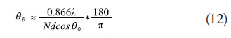
Where N is the number of elements.
The second test is made by taking the Matlab® “linear_array.m” function as reference, introduced by Bassem R. Mahafza in the work “Radar Systems Analysis and Design Using Matlab®” where the radiation pattern can be observed for a linear antenna.
The parameters measured to test the functioning are: width of the main lobe measured in degrees, the peak power in each of the lobes normalized to one, and the pointing angle for each lobe. For this, the measurements for the pointing angles of the main lobe are taken from 0 to 90°, in 10° leaps, measured from the perpendicular to the antenna. The following are the results obtained:
As noted in Figure 9, the results obtained by the three methods are very close up to a 30° pointing angle, even similar up to a 60° angle. As of 60°, it can be noted how the approximation proposed by Skollnick increases exponentially. The author clarifies in his work that the approximation operates for angles below 60°. Regarding the results of the “linear_ array .m” function, compared to those of the “3D” program, it may be observed that they are almost identical. It is worth clarifying that both methods reach their respective results via different methods. The “linear_array.m” function employs the discrete fast Fourier transform, from the lighting function, while the “3D” program employs the sum of all the electric fields in each point.
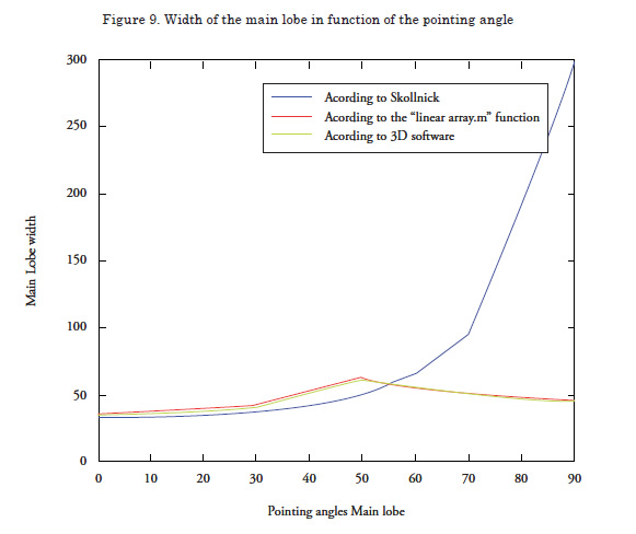
Peak Power normalized to one in function of the Pointing Angle
The magnitude of the peak power in each of the lobes is normalized and is compared with respect to the peak power of the main lobe. This is a very useful parameter to determine the relationship between the main lobe and the side lobes. As can be observed in Figure 10, the data taken in the “linear_ array .m” and the “3D” program are almost identical.
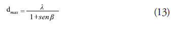
Pointing Angle of each lobe
By measuring the pointing angle of each lobe, we can confirm that the main lobe points in the desired direction. In addition to visualizing that the results obtained by both methods are quite similar.
Distance between elements
This parameter is especially important in the design of arrays because the separation of the elements permits narrower phases but generates greater height in the side lobes. The optimal spacing should produce narrow phase widths and small side lobes with a minimum of elements. It is also necessary to determine what will be the maximum pointing angle we want to achieve, given that with greater pointing angle greater side lobes and less width of the main lobe.
This ratio is suggested by Stimson G. [3] with the following equation.
Where dmax is the maximum gap between elements, and β is the maximum pointing angle sought. Figure 12 shows the solution to the equation for pointing angles between 0° and 90°. From the graphic, it may be deduced that for gap separations below 0.5 wavelengths, the maximum pointing angle is not limited, and that for gaps greater than a wavelength, there will always be side lobes important for pointing angles different to zero.
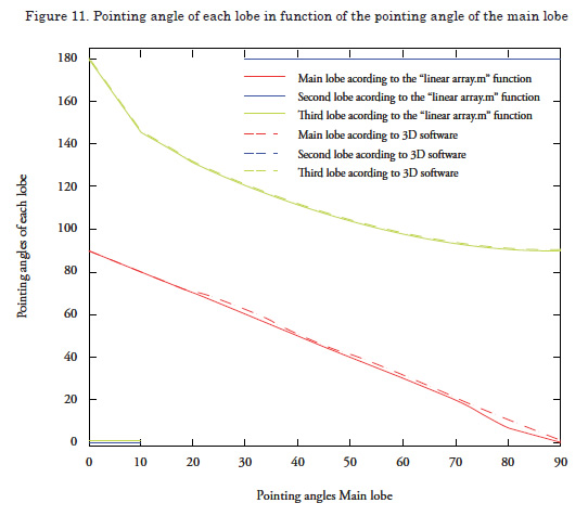
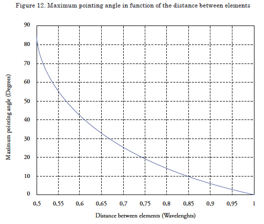
Figure 13 shows the results of the measurements of the amplitudes of the biggest side lobes for the different gaps between elements pointing the phase in different directions. It may be confirmed that the when the gap is greater between elements, the big side lobes appear in the smaller pointing angles.
Note that for 0.5 wavelength gaps, and pointing angles above 70° there are big side lobes, implying that the rule exposed by Stimson is not fulfilled. However, we were able to show that upon increasing the antenna length, the maximum pointing angle for gaps of 0.5 wavelengths increases with a tendency to reaching 90°, suggesting that the equation exposed by Stimson supposes an antenna of infinite length in which case the condition would be fulfilled.
Plannar Antenna
For planar antennas, proceed to verify their performance by varying length and effective area of the antenna, shape of the array, disposition of the elements in the array, the directivity of each element, distance between elements, the lighting function, granularity, and the pointing angle. The parameters to be measured will be: the percentage of power concentrated in each lobe, the peak power of each lobe, the ratio in decibels of the side lobes with respect to the main lobe, the directive gain, measurements in degrees, at points of half power, from the main lobe in the vertical and horizontal senses, and the solid angle formed by these measurements.
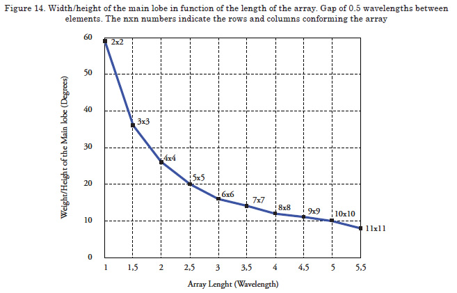
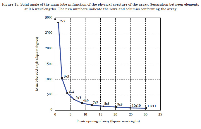
Length and effective area of the Antenna
According to theory, as the length of the antenna is increased with respect to the wave length, the main lobe will become narrower. To confirm that the program behaves according to these parameters, measurements will taken for rectangular arrays conformed of 2x2 to 11x11 omnidirectional elements, with vertical and horizontal gaps of 0.5 wavelengths between elements, uniform lighting function, disposition in cross shape, and a 0° pointing angle. Antenna length is given by the number of elements and the gap between them. As noted in Figure 14, the condition posed is fulfilled, given that the greater antenna length will make the main lobe narrower. Analogically, it is shown that the condition is fulfilled for the physical aperture of the antenna, having to diminish the solid angle of the main lobe when increasing the area of the antenna, as observed in Figure 15.
The Lighting Function
This parameter is quite important in regards to the suppression of side lobes. It consists in controlling the signal width of each element. Knowing that the radiation pattern in the far field is an approximation to the Fourier transform of lighting function, we can then approach the shape of the radiation pattern by controlling the lighting function.
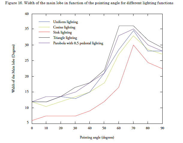
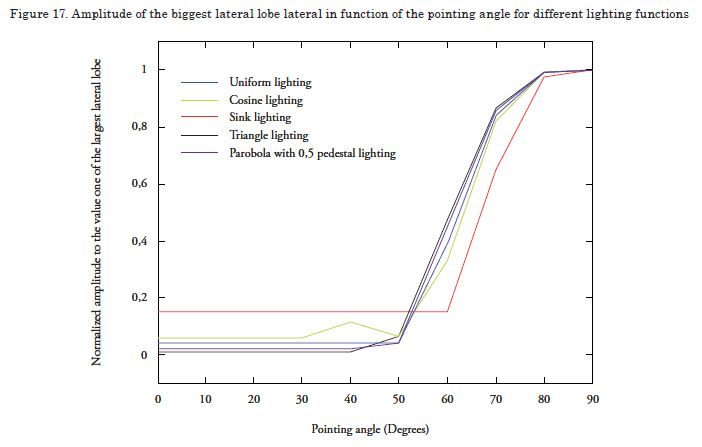
To test the functioning, use an array of 10 x 10 elements, in circular shape, with gap of 0.5 wavelengths, with different pointing degrees and alternating the lighting function among uniform, triangular, parabolic, cosine, and sink. In each case, evaluate the width of the main lobe and the height of the biggest secondary lobe.
Upon observing Figure 16, it may be deduced that the best lighting function to accomplish a narrow phase width is a “sink” function and the worst is the triangular function.
Upon observing Figure 17, it may be deduced that the best lighting function to accomplish small side lobes is the triangular function and the worst is the “sink” function. From the two previous deductions, we may state that there is a commitment between the width of the main lobe and the height of the side lobes, which besides depending on the gap between elements, also depends on the lighting function.
The selection of the lighting function will then depend on the specific requirements of the particular application.
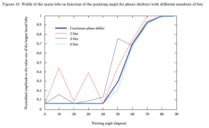
Granularity and the Pointing Angle
This parameter permits visualizing the effect the phase shifters of binary or digital functioning have on phase pointing. For such, we will use an array of 5 x 5 elements, of rectangular shape, with uniform lighting function, gap between elements of 0.5 wavelengths, employing phase shifters from 1 to 5 bits for the different pointing angles. The width of the main lobe and the amplitude of the biggest secondary lobe will be measured to test the functioning.
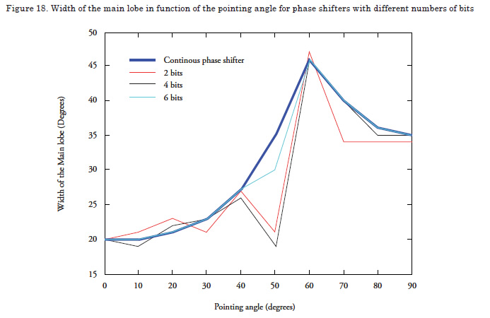
As noted in Figures 18 and 19, as the number of bits of the phase shifter is increased, the performance of the array appears more like when a continuous phase shifter is used. Observe how the side lobes are increased while the main lobe is broadened or narrowed when trying to point the phase in certain directions with a limited number of bits (red line = 2 bits). It is also noted that by using 6 bits, the response of the side lobes and the main lobe is quite similar to that of the continuous phase shifter.
Directivity of each Element
This parameter permits employing elements with distinct radiation patterns; this serves to visualize the functioning of more realistic arrays and will permit – in case of having the measurements – incorporating data of real elements and, thus, visualizing how said elements would behave in distinct dispositions.
Shape and disposition of the Elements in the Array
These two aspects that can be manipulated in the program represent a good number of possibilities and their effect on the performance of the array is quite complex; thereby, they will not be used in this work as proof. However, given that they are enabled within the program, they permit future research on the theme.
Problem of exercise
To show the use of the program as a tool for the design of an active phased array, a hypothetical design problem is posed and a solution is sought.
Let us suppose that we need to design an active phased array antenna for a radar that must comply with the following specifications: Electronically steer the phase in vertical sense with a beam 3° in width and 3 decibels in the horizontal and 15° in the vertical, able to have a pointing angle of ± 50° in vertical sense, operate in the G band, employ the least possible elements and be the smallest possible size, have small side lobes and be steerable in elevation in 3-degree steps without important degradation of its radiation pattern.
Employing the approach suggested by Skollnik in [2], which indicates that for an array of “N” elements with a gap of 0.5 λ between elements, the width of the main lobe in ![]() half power is:
half power is:
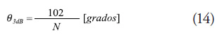
The number of elements that would be necessary to comply with the required widths of the main lobe may be estimated, both in the vertical and horizontal sense.
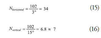
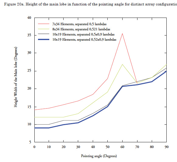
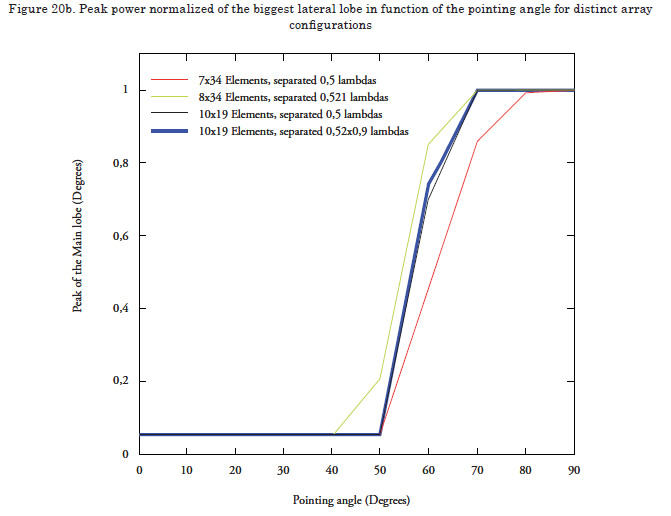
Then, an array is constructed with 7 x 34 elements, initially with cross-shaped disposition and rectangular shape, uniform lighting function, gap between elements of 0.5 wavelengths, and continuous phase shifters. Given the lack of knowledge of the radiation pattern of the elements, these are presumed omnidirectional. Thereafter, the configuration is modified in function of the results obtained increasing the antenna length by adding another element and vertically increasing the distance between elements up to 0.521 wavelengths; this with the purpose of diminishing the height of the main lobe. It is noted that height diminishes but without complying with the required specifications. Because of the aforementioned, we proceed to add another element in vertical sense until completing 10 rows; additionally, the distance between elements is increased in horizontal sense up to 0.9 wavelengths and the number of elements is decreased to 19 per row, seeking to maintain the antenna length; bearing in mind that electronic phase steering is not required in the horizontal sense.
The results obtained indicate that to accomplish the required specifications, a configuration of 10x19 elements is required with vertical gap of 0.52 wavelengths and horizontal gap of 0.9 wavelengths. These results correspond to the blue line in Figure 20.
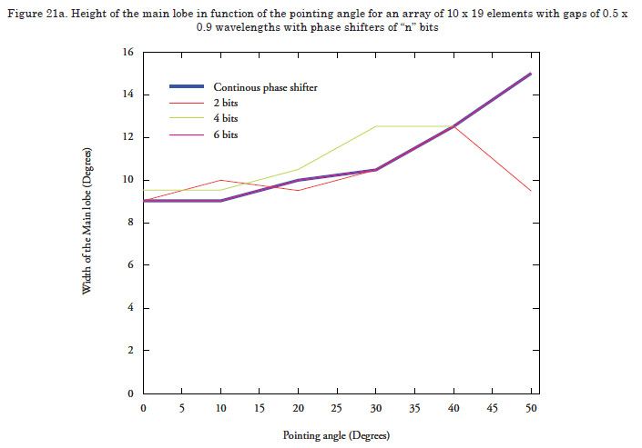
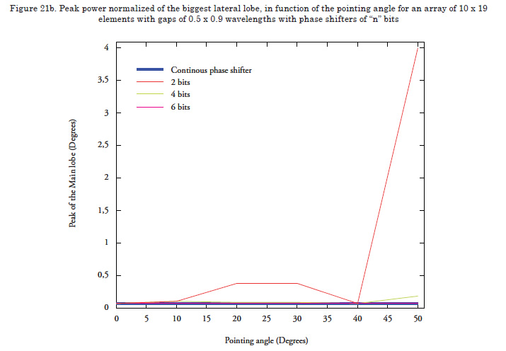
Now the required granularity configuration will be sought, taking values from 2 bits until reaching a number where results are accomplished within the parameters.
The results observed in Figure 21 indicate that phase shifters are required with 4 bits to accomplish satisfactory performance.
Conclusions
It is useful to model the theoretical functioning of a phased array by employing computer tools like Matlab®, given that it represents savings in costs during the initial stages of the design, permitting the visualization of problems and prevention of errors prior to the physical construction of prototypes.
Phased-active arrays are the present and future of radiofrequency antennas because they offer great advantages, among which the most important are the extreme agility to steer the phase, which permits almost instantaneous spatial multiplexing.
As conclusion of the proof, it may be stated that the measurements made with the “3D” program adjust to the models used as reference, which are presumed approximate to the reality given the trajectory of its authors. Hence, the model employed is suitable to model antenna arrays.
Bibliography
[1] KRAUS JOHN D., MARTHEFKA RONALD J. Antennas for all applications, third edition .Chapter 4 Point source.P72-86. Chapter 5 Arrays of point sources. P 90-159.
[2] SKOLLNICK, MERRILL L. Introduction to radar systems, third edition. Mc Graw Hill. Chapter 9. The Radar Antenna. 9.5 Electronically Steered Phased Array Antennas. P559-566. 9.6 Phase Shifters. P567-580. 9.8 Radiators for Phased Arrays. P589-593. 9.9 Architectures for Phased arrays. P594-614. 9.14. Cost of Phased Array Radar. P646-650. 9.16 Systems Aspects of Phased Array Radars. P658-660.
[3] STIMSON GEORGE W. Air-Born Radar, Second edition. Science Publishers INC. Part IX Advanced Concepts. Chapter 37. Electronically Steered array antennas. P473- 479. Chapter 38. ESA design. P481-498.
[4] EDDE, BYRON. Radar Principles Technologies and Applications. Practice Hall PTR. Chapter 9 Radar Antennas. 9-2 Arrays of discrete elements- Principles. P422-426. 9-8 Electronically Phased steered Arrays. P450- 460.
[5] BASSEM R. MAHAFZA. Radar Systems Analysis and Design using Matlab®, Second Edition. Chapman & Hall/CRC. 2005.
1Set of particles with common origin, which propagate without dispersion. Microsoft® Encarta® 2008. © 1993-2007 Microsoft Corporation. All rights reserved.