Application of Sampling Based Model Predictive Control to an Autonomous Underwater Vehicle

Charmane V. Caldwell¹
Damion D. Dunlap²
Emmanuel G. Collins Jr.³

Abstract

Unmanned Underwater Vehicles (UUVs) can be utilized to perform difficult tasks in cluttered environments such as harbor and port protection. However, since UUVs have nonlinear and highly coupled dynamics, motion planning and control can be difficult when completing complex tasks. Introducing models into the motion planning process can produce paths the vehicle can feasibly traverse. As a result, Sampling-Based Model Predictive Control (SBMPC) is proposed to simultaneously generate control inputs and system trajectories for an autonomous underwater vehicle (AUV). The algorithm combines the benefits of sampling-based motion planning with model predictive control (MPC) while avoiding some of the major pitfalls facing both traditional sampling-based planning algorithms and traditional MPC. The method is based on sampling (i.e., discretizing) the input space at each sample period and implementing a goal-directed optimization (e.g., A*) in place of standard numerical optimization. This formulation of MPC readily applies to nonlinear systems and avoids the local minima which can cause a vehicle to become immobilized behind obstacles. The SBMPC algorithm is applied to an AUV in a 2D cluttered environment and an AUV in a common local minima problem. The algorithm is then used on a full kinematic model to demonstrate the benefits.

Key words: Motion planning, path planning, model predictive control, sampling, autonomous underwater vehicles.

Resumen

Los UUVs pueden ser utilizados para realizar tareas difíciles en ambientes atiborrados de reflexiones de onda tales como muelles y puertos. Sin embargo, dado que los UUVs tienen dinámicas áltamente acopladas y no lineales, la programación de movimiento y el control pueden ser complicados cuando son realizadas tareas complejas. Introducir modelos en el proceso de programación del movimiento puede producir patrones que el vehículo puede cruzar de manera viable. Como resultado, el modelo de control predictivo basado en muestreo (SBMPC, por sus siglas en inglés) es propuesto para generar simultáneamente entradas de control y trayectorias de sistema para un vehículo autónomo sumergible. El algoritmo combina los beneficios de la planeación de movimiento con el control predictivo de modelo (MPC), mientras que evita algunos de los mayores obstáculos que enfrentan tanto los algoritmos basados en muestreo como el tradicional MPC. El método está basado en el muestreo (es decir, discretización) del espacio de entrada en cada período de muestreo e implementación de una optimización dirigida a objetivos (por ejemplo, A*) en lugar de la optimización numérica estándar. Esta formulación del MPC aplica fácilmente a los sistemas no lineales y evita el mínimo local, el cual puede ocasionar que un vehículo quede inmóvil detrás de los obstáculos. El algoritmo SBMPC se aplica a un UAV en un ambiente cargado de reflexiones de onda y a un UAV en un problema de mínimo común local. El algoritmo es luego usado en un modelo cinemático completo para demostrar los beneficios de aplicar restricciones y un modelo en programación de movimiento.

Palabras claves: Programación de movimiento, programación de ruta, Modelo de control predictivo, muestreo, Vehículo Autónomo Subacuático.

Date received: May 21th, 2010. - Fecha de recepción: 21 de Mayo de 2010.
Date Accepted: July 6, 2010. - Fecha de aceptación: 6 de Julio de 2010.

________________________

¹ Department of Electrical and Computer Engineering CISCOR of the FAMU-FSU COE. Florida. U.S.A. e-mail: cvcaldwe@eng.fsu.edu
² Naval Surface Warfare Center. Panama City, FL. U.S.A. e-mail: damion.d.dunlap@navy.mil
³ Department of Electrical and Computer Engineering CISCOR of the FAMU-FSU COE. Florida. U.S.A. e-mail: ecollins@eng.fsu.edu

............................................................................................................................................................

Introduction

The United States has over 360 ports that comprise more than 90% of the U.S. export and import industry [1]. These harbors pass through cargo and even passengers. A threat to the ports can produce an environmental and economic crisis [2]. A simple tactic a terrorist can use to cause havoc is employing mines or maritime improvised explosive devices (MIEDs) at a U.S. port. In this way a mine that cost no more than a few thousand dollars can cause great disruption. There have been non-mine related crises in the past that have caused setbacks at U.S. ports: the Exxon Valdez spill of 1989, which cost more than $2.5 billion to clean up, and the dock workers strike of 2002, which resulted in a loss of $1.9 billion dollars a day [2]. The effect of closing a port due to a mine explosion can also be catastrophic.

Consequently, it is necessary to protect U.S. ports. The task of searching and destroying mines is a dangerous process that can be performed by a combination of surface vehicles, unmanned underwater vehicles (UUVs), and explosive ordinance divers (EODs) [1]. This paper will consider the use of an UUV, more specifically an autonomous underwater vehicle (AUV). Harbors and ports have naval ships, commercial vessels, fishing boats, piers and other articles that create a cluttered environment for AUV motion. For the inspection to be successful the AUV cannot collide with an obstacle, because this can obviously be very disruptive. In addition to the complex AUV mobility environment, the nonlinear, timvarying and highly coupled vehicle dynamics make motion planning and control difficult for harbor protection tasks since it is difficult to predict future paths for the vehicle as it moves through the environment. In addition, there are uncertainties in the hydrodynamic coefficients determined in a tank test, which effect the confidence in the fidelity of the dynamic model when the AUV maneuvers in the ocean. The vehicle is underdamped and easily perturbed, which is a challenge when there are external disturbances like ocean currents that cause the vehicle to deviate from its path. Furthermore, the center of gravity and buoyancy may change depending on the AUV payload. Consequently, an AUV requires robust motion planning and control to operate reliably in complex environments.

Standard AUV motion planning and control first determines a trajectory that the AUV may not be physically able to follow, then applies a controller that may require the vehicle to follow this possibly infeasible trajectory. An approach that can help ensure robust motion planning is to incorporate a model of the AUV when planning the vehicle trajectory since this applies motion constraints that ensure feasible trajectories. In cluttered environments, the use of kinodynamic constraints in motion planning aid in determining a collision free trajectory. The kinematics provides the turn rate constraint and side slip [3], while the dynamics can provide insight into an AUV’s movement and interaction with the water, providing limits on velocities, accelerations and applied forces. This paper presents results for motion planning with a kinematic model. A future paper will consider planning using an AUV dynamic model.

There are researchers that have previously incorporated a model in motion planning for an AUV. Kawano has a four part system [4]: 1) the offline Markov Decision Process module performs the motion planning offline; 2) the replanning module determines a path when there are new obstacles; 3) the realtime path tracking module gives action that needs to be taken; 4) the feedback control module regulates the vehicles’ velocity to the target velocity. Yakimenko uses the direct method of calculus to generate trajectories that are kinematically feasible for the vehicle to traverse [5]. There are four main blocks: the first generates a candidate trajectory that satisfies boundary conditions and position, velocity and acceleration constraints; the second employs inverse dynamics to determine the states and control inputs necessary to follow the trajectory; the third computes states along the reference trajectory over a fixed number of points; and the fourth optimizes the performance index.

The current line of research first considered using the model in the motion planning process by integrating the guidance and control via a method called shrinking horizon model predictive control [6]. That approach was often able to determine a collision free path using a kinematic model, but had two primary shortcomings. First, the computational time was not fast enough for real time vehicle operation. Second, for certain initial condition the gradient-based optimization method would converge to a local minimum. To solve these issues Sampling Based Model Predictive Control (SBMPC) was developed [7].

SBMPC allows a model to be considered online while simultaneously determining the optimal control input and a kinematically or dynamically feasible trajectory of the AUV. SBMPC is a nonlinear model predictive control (NMPC) algorithm that can avoid local minimum, has strong convergence properties based on the LPA* optimization convergence proof [8], and has physically intuitive tuning parameters. The concept behind SBMPC was first presented in [7]. A more developed version that tested SBMPC on an Ackerman Steered vehicle [9] was later presented. As its name implies, SBMPC is dependent upon the concept of sampling, which has arisen as one of the major paradigms for robotic motion planning [10]. Sampling is the mechanism used to trade performance for computational efficiency. Unlike traditional model predictive control (MPC), which views the system behavior through the system inputs, the vast majority of previously developed sampling methods plan in the output space and attempt to find inputs that connect points in the output space. SBMPC is an algorithm that, like traditional MPC, is based on viewing the system through its inputs. However, unlike previous MPC methods, it uses sampling to provide the trade-off between performance and computational efficiency. Also, in contrast to previous MPC methods, it does not rely on numerical optimization. Instead it uses a goal-directed optimization algorithm derived from LPA* [8], an incremental A* algorithm [10].

This paper is arranged as follows. Section II provides a summary of the methods combined to formulate SBMPC. The SBMPC algorithm is presented in Section III. Section IV gives twodimensional simulations of SBMPC implemented on AUVs in clustered environments and local minima configurations. Then a three-dimensional simulation in free space is provided. Finally, Section V presents conclusions and future work.

The Fundamentals of Sampling Based Model Predictive Control

SBMPC is a novel approach that allows real time motion planning that uses the vehicle’s nonlinear model and avoids local minima. The method employs an MPC type cost function and optimizes the inputs, which is standard in the control community. Instead of using traditional numerical optimization, SBMPC applies sampling and a goal-directed (A* -type) optimization, which are standard in the robotic and AI communities. This section provides a brief overview of the methods from which SBMPC was derived. Next, it describes the SBMPC cost function and outlines the SBMPC algorithm. Finally, this section disusses the benefits of SBMPC.

Model Predictive Control

Introduced to the process industry in the late 1970s [11], Model Predictive Control (MPC) is a mixture of system theory and optimization. It is a control method that finds the control input by optimizing a cost function subject to constraints. The cost function calculates the desired control signal by using a model of the plant to predict future plant outputs. MPC generally works by solving an optimization problem at every time step k to determine control inputs for the next N steps, known as the prediction horizon. This optimal control sequence is determined by using the system model to predict the potential system response, which is then evaluated by the cost function J. Most commonly, a quadratic cost function minimizes control effort as well as the error between the predicted trajectory and the reference trajectory, r. The prediction and optimization operate together to generate sequences of the controller output u and the resulting system output y. In particular, the optimization problem is

subject to the model constraints,

and the inequality constraints,

Traditional MPC has typically been computationally slow and incorporates simple linear models.

Sampling Based Motion Planning

Sampling-based motion planning algorithms include Rapidly-exploring Random Tree (RRTs) [12], probability roadmaps [13], and randomized A* algorithms [14]. A common feature of each of those algorithms to date is that they work in the output space of the robot and employ various strategies for generating samples (i.e., random or pseudorandom points). In essence, as shown in Fig. 1, sampling-based motion planning methods work by using sampling to construct a tree that connects the root with a goal region. Th e general purpose of sampling is to cover the space so that the samples

are uniformly distributed, while minimizing gaps and clusters [15].

Goal Directed Optimization

Th ere is a class of discrete optimization techniques that have their origin in graph theory and have been further developed in the path planning literature. In this paper these techniques will be called goal-directed optimization and refer to graph search algorithms such as Dijkstra’s algorithm and the A*, D*, and LPA* algorithms [10], [8]. Given a graph, these algorithms fi nd a path that optimizes some cost of moving from a start node to some given goal. Although not commonly recognized, goal-directed optimization approaches are capable of solving control problems for which the ultimate objective is to generate an optimal trajectory and control inputs to reach a goal (or set point) while optimizing a cost function; hence, they apply to terminal constraint optimization problems and set point control problems.

The SBMPC Optimization Problem

SBMPC overcomes some of the shortcomings of traditional MPC by sampling the input space as opposed to sampling the output space as in traditional sampling-based motion planning methods. Th e need for a nearest-neighbor search is eliminated and the local planning method (LPM) is reduced to the integration a system model and therefore only generates outputs that are achievable by the system. To understand the relationship between sampling-based algorithms and MPC optimization, it is essential to pose samplingbased motion planning as an optimization problem. To illustrate this point, note that, subject to the constraints of the sampling, a goaldirected optimization algorithm can eff ectively solve the mixed integer nonlinear optimization problem,

subject to the system equations,

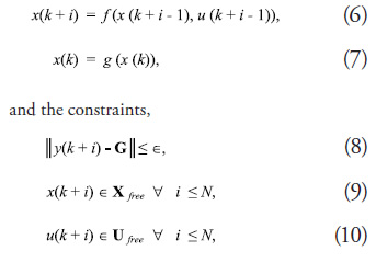
where Δu(k + i) = u(k + i) - u(k + i - 1), Q(i) ≥ 0, S(i) ≥ 0, and Xfree and represent the states and inputs respectively that do not violate any of the problem constraints. The term represents the edge cost of the path between the current predicted output y(k + i) and the next predicted output y(k + i + 1). The goal state G is represented as a terminal constraint as opposed to being explicitly incorporated into the cost function. Goal-directed optimization methods implicitlyconsider the goal through the use of a function that computes a rigorous lower bound of the cost from a particular state to G. This function, often referred to as an “optimistic heuristic” in the robotics literature, is eventually replaced by actual cost values based on the predictions and therefore does not appear in the final cost function. The cost function can be modified to minimize any metric as long as it can be computed as the sum of edge costs.

The SBMPC ALGORITHM

The formal SBMPC algorithm can be found in [9]. However, the main component of the SBMPC algorithm is the optimization, which will be called Sampling-Based Model Predictive Optimization and consists of the following steps:

1. Sample Control Space: Generate a set of samples of the control space that satisfy the input constraints.
2. Generate Neighbor Nodes: Integrate the system model with the control samples to determine the neighbors of the current node.
3. Evaluate Node Costs: Use an A* -like heuristic to evaluate the cost of the generated nodes based on the desired objective (shortest distance, shortest time, or least amount of energy, etc.).
4. Select Lowest Cost Node: The nodes are collected in the Open List, which ranks the potential expansion nodes by their cost. The Open List is implemented as a heap so that the lowest cost node that has not been expanded is on top.
5. Evaluate Edge Cost for the “Best” Node: Evaluate each of the inequality constraints described in (6) for the edge connecting the “best” node to the current node. The edge cost evaluation requires sub-sampling and iteration of the model with a smaller time step for increased accuracy; it is therefore only computed for the current “best”node. In the worst case the edge cost of all of the neighbor nodes will be evaluated, which is how A* typically computes cost.
6. Check for Constraint Violations: If a constraint violation occurred, go back to step 4 and get the next “best” node.
7. Check for Completion: Determine if the current solution contains a path to the goal. If yes, stop. If no, go back to step 1.

The entire algorithm is integrated into the MPC framework by executing the first control and repeating the optimization until the goal is reached since the completion of SBMPO represents the calculation of a path to the goal and not the complete traversal.

Benefits of SBMPC

The novel SBMPC approach has several benefits. First, SBMPC is a method that can address problems with nonlinear models. It effectively reduces the problem size of MPC by sampling the inputs of the system, which considerably reduces the computation time. In addition, the method also replaces the traditional MPC optimization phase with LPA*, an algorithm derived from A* that can replan quickly (i.e., it is incremental). SBMPC retains the computational efficiency and has the convergence properties of LPA* [8], while avoiding some of the computational bottlenecks associated with sampling-based motion planners. Lastly, tuning for this method requires choosing the number of samples and the implicit state grid resolution, which are physically intuitive parameters.

SBMPC Simulation Results

The results presented in this section have three purposes: 1) to demonstrate how SBMPC can handle AUVs moving in cluttered environments, 2) to demonstrate how the SBMPC algorithm behaves when a local minimum is present and the effect sampling has on the optimal solution, and 3) to show how the inclusion of constraints and a model in motion planning can produce a feasible path. It is assumed the obstacle information is available to the SBMPC algorithm. The problems associated with the uncertainty in sensing obstacles are beyond the scope of this paper. However, it must be addressed for real world implementation of SBMPC on AUVs.

SBMPC Motion Planning for an AUV in Cluttered Environments

Motion planning for an AUV moving in the horizontal plane is developed using the 2-D kinematic model,

where the inputs u and r are respectively the forward velocity along the x-axis and angular velocity along the z-axis. Consequently, there are two inputs and three states in this model. The velocity u was constrained to lie in the interval (0 2) m/s, and the steering rate ψ was constrained to the interval (-15° 15°) rad/s.

The basic problem is to use the kinematic model (11) to plan a minimum-distance trajectory for the AUV from a start posture (0m; 0m; 0°) to a goal point (20m; 20m) while avoiding the numerous obstacles of a cluttered environment.

The parameters for the simulations are shown in Table 1. It is assumed that the time step in the SBMPC cost function (5) is Tc. For SBMPC the constraints were checked every time the model was updated corresponds to the period over which the control inputs were held constant. There were 100 simulations in which 30 obstacles of various sizes and locations were randomly generated to produce different scenarios. As a result, in Table 1 the prediction horizon varies because each random scenario requires a different number of steps to traverse from the start position to the goal position. In each simulation the implicit state grid resolution was 0.1m. SBMPC was used to solve the optimization problem (5) - (10) with Q(i) = I and S(i) = 0 and yielded the optimal number of steps N* in addition to the control input sequence.

The results of 100 random simulations on a 2 GHz Intel Core 2 Duo Laptop are shown in Table 2. Representative results from the 100 scenarios are shown in Figs. 2 and 3. These are typical scenarios which show SBMPC’s ability to create a kinematically feasible trajectory in a complex environment without getting stuck in a local minimum. In the figures a circle on the path curve represents the predicted output of the vehicle that coincides with the optimal sampled input. In Fig. 2 the inputs are sampled more as the vehicle comes close to a cluster of obstacles or a large obstacle. Fig. 3 demonstrates how the AUV overcomes a large cluster of obstacles at the start of a mission. As shown in Table 2, the AUV was able to reach the goal in each of the 100 cluttered environment

simulations. Th is is important since true autonomy requires a vehicle to be able to successfully complete a mission on its own. Note there is an order of magnitude diff erence in the mean CPU time and median CPU time of Table 2, because a few of the randomly generated scenarios had obstacles clustered to form larger obstacles, which creates computationally intensive planning problems.

SBMPC Motion Planning for an AUV in Cluttered Environments

As stated previously, SBMPC can handle local minimum problems that other methods have diffi culties handling. In this section SBMPC is used to solve a common local minimum problem in which the vehicle has a concave obstacle in front of the goal. Note that whenever the vehicle is behind an obstacle or group of obstacles and has to increase its distance from the goal to achieve the goal, it is in a local minimum position. Th e parameters for these simulations are given by Table 1 with the exception that the number of samples for the simulation of Fig. 5 was increased from 10 to 25. Th e vehicle has a start posture of (5m; 0m; 90°) and the goal position (5m; 10m).

SBMPC introduces suboptimality through its sampling of the inputs. As the number of samples of the input space increases the solution optimality increases at the expense of increased computational time. In Figs. 4 and 5 the AUVs approach the composite concave obstacle but determines a path around it to the goal. Even though, both AUVs reach the goal, because Fig. 5 uses a larger number of input samples than Fig. 4 the solution path is shorter (i.e. more optimal). This increase in the number of samples comes with a price. The path of Fig. 4, which was based on 10 samples, requires 1:0s to determine a path, but the path of Fig. 5, based on 25 input samples, has a computation time of 12:7s. To achieve an algorithm that can be implemented online there are trade offs between speed and optimality. It is important to determine a balance between the two.

SBMPC Motion Planning for an AUV in 3D Environment

Motion planning in a 3D environment uses the full kinematic model of the AUV,

where u, v, w are linear velocities in the local body fixed frame along the x, y, z axes, respectively and p, q, r are the angular velocities in the local body fixed frame along the x, y, z axes, respectively. The AUV posture can be defined by six coordinates, 3 representing the position and 3 corresponding to the orientation , all with respect to the world frame. The variable constraints are provided in Table 1.

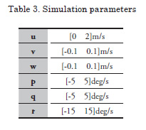
For this simulation the sampling factor was 25. A start posture of (12m, 0m, -5m, 0°, 0°, 0°) was given with a goal point of (0m, 0m, -5m, ), which is directly behind the start point. Since the vehicle was constrained to forward velocity along the x-axis it could not reverse to the goal. As Fig. 6 shows, it must turn around to reach the goal. A path planner that considers a vehicle to be holonomic would simply produce a straight line from the start to the goal. However, the ability of SBMPC to consider the vehicle constraints and kinematic model produces a feasible trajectory from the start to the goal.

Conclusions

Sampling-Based Model Predictive Control has been shown to effectively generate a control sequence for an AUV in the presence of a number of nonlinear constraints. SBMPC exploits samplingbased concepts along with the LPA* incremental optimization algorithm to achieve the goal of being able to quickly determine control updates while avoiding local minima. The SBMPC solution is globally optimal subject to the chosen sampling method. When the entire state space is gridded, the SBMPC algorithm guarantees that the algorithm will converge to a solution if one exists.

This paper presents preliminary results using the 2D kinematic model in cluttered environments and a 3D kinematic model in free space. A future goal of this research is to consider 3-D motion utilizing the dynamic model. However, a dynamic model has greater complexity then a kinematic model, which will lead to increased computational times, and difficulties in achieving real time operation. One possible solution is to employ a method that switches from a dynamic model in complex situations to a kinematic model in less complex circumstances.

Currently, the goal region is only concerned with the AUV reaching a certain position. However, in certain missions, such as docking or recovery, it may be necessary for the vehicle to arrive at a specified posture. Consequently, the goal region will include the orientation in future work.

Lastly, because of the constantly changing environment in which the AUV must move, the time varying nature of the AUV dynamics, and the uncertainty of the hydrodynamic coefficients it is important to eventually replan the path. This is one of the benefits of traditional MPC; by replanning at every time step it produces robustness. SBMPC can incorporate replanning through the use of LPA*.

References

[1] S. TRUVER, “Mines, improvided explosives: a threat to global commerce?” National Defense Industrial Association, vol. 91, no. 641, pp. 46–47, April 2007.

[2] A. WILBY, “Meeting the threat of maritime improvised explosive devices,” Sea Technology, vol. 50, no. 3, March 2009.

[3] M. CHERIF, “Kinodynamic motion planning for all-terrain wheeled vehicles,” Proceeding IEEE International Conference on Robotic and Automation, pp. 317–322, 1999.

[4] H. KAWANO, “Real-time obstacle avoidance for underactuated autonomous underwater vehicles in unknown vortex sea flow by the mdp approach,” International Conference on Intelligent Robots
and Systems, pp. 3024–3031, October 2006.

[5] O. YAKIMENKO, D. HORNER, and D. P. Jr., “Auv rendezvous trajectories generation for underwater recovery,” Mediterranean Conference on Control and Automation, pp.
1192–1197, June 2008.

[6] C. CALDWELL, E. COLLINS, and S. PALANKI, “Integrated guidance and control of auvs using shrinking horizon model predictive control,” OCEANS Conference, September 2006.

[7] D. D. DUNLAP, E. G. COLLINS, JR., and C. V. CALDWELL, “Sampling based model predictive control with application to autonomous vehicle guidance,” Florida Conference on Recent Advances in Robotics, May 2008.

[8] S. KOENIG, M. LIKHACHEV, and D. FURCY, “Lifelong planning A*,” Artificial Intelligence, 2004.

[9] D. DUNLAP, C. CALDWELL, and E. COLLINS, “Nonlinear model predictive control using sampling and goal-directed optimization,” IEEE Multiconference on Systems and Control, September 2010.

[10] S. M. LAVALLE, Planning Algorithms. Cambridge University Press, 2006.

[11] J. MACIEJOWSKI, Predictive Control with Constraints. Haslow, UK: Prentice Hall, 2002.

[12] S. M. LAVALLE, “Rapidly-exploring random trees: A new tool for path planning,” Iowa State University, Tech. Rep., 1998.

[13] L. E. KAVRAKI, P. SVESTKA, J. C. LATOMBE, and M. H. OVERMARS, “Probabilistic roadmaps for path planning in high-dimensional configuration spaces,” IEEE Transactions on Robotics & Automation, vol. 12, no. 4, pp. 566 – 580, June 1996.