Metamodeling Techniques for Multidimensional Ship Design Problems

Peter B. Backlund ¹
David Shahan ²
Carolyn C. Seepersad ³

Abstract

Metamodels, also known as surrogate models, can be used in place of computationally expensive simulation models to increase computational efficiency for the purposes of design optimization or design space exploration. Metamodel-based design optimization is especially advantageous for ship design problems that require either computationally expensive simulations or costly physical experiments. In this paper, three metamodeling methods are evaluated with respect to their capabilities for modeling highly nonlinear, multimodal functions with incrementally increasing numbers of independent variables. Methods analyzed include kriging, radial basis functions (RBF), and support vector regression (SVR). Each metamodeling technique is used to model a set of single-output functions with dimensionality ranging from one to ten independent variables and modality ranging from one to twenty local maxima. The number of points used to train the models is increased until a predetermined error threshold is met. Results show that each of the three methods has its own distinct advantages.

Key words: Metamodeling, kriging, radial basis functions, support vector regression, metamodel-based design optimization.

Resumen

Los metamodelos, también conocimos como modelos substitutos, pueden ser utilizados en lugar de modelos cuyas simulaciones tienen un costo computacional muy alto, incrementado con esto la eficiencia en procesos de optimización de diseños o en el diseño de exploraciones espaciales. La optimización de diseños basados en metamodelos es especialmente ventajosa en problemas de diseño relacionado con vehículos marinos en los cuales se requieran simulaciones con un alto costo computacional o bien de experimentos con una alta inversión en equipos. En este artículo se evalúan tres métodos para el desarrollo de metamodelos. La evaluación de estos métodos es desarrollada teniendo en cuenta la capacidad de cada uno de ellos para modelar funciones multimodales no lineales con un número creciente de variables independientes. Dentro de los métodos analizados se encuentran el método de kriging, el método de funciones de base radiales, y el método de regresión con vector de apoyo. Cada una de las anteriores técnicas para la generación de metamodelos es utilizada para modelar un grupo de funciones de una salida con dimensiones variando desde uno hasta diez variables independientes y una modalidad variando entre uno y veinte máximos locales. El número de puntos utilizados para entrenar los modelos es incrementado hasta que el error alcanza una tolerancia predeterminada. Los resultados obtenidos muestran que cada uno de los tres modelos tiene sus propias ventajas distintivas.

Palabras claves: Desarrollo de metamodelos, kriging, funciones de base radiales, regresión con vector de apoyo, optimización de diseños basada en metamodelos.

Date received: May 19th, 2010. - Fecha de recepción: 19 de Mayo de 2010.
Date Accepted: July 6, 2010. - Fecha de aceptación: 6 de Julio de 2010.

________________________

¹ Applied Research Laboratories. The University of Texas. Austin, TX. USA. e-mail: pbacklund@mail.utexas.edu
² The University of Texas. Austin, TX. USA. e-mail: david.shahan@mail.utexas.edu
³ The University of Texas. Austin, TX. USA. e-mail: ccseepersad@mail.utexas.edu

............................................................................................................................................................



Introduction

Computer models of naval systems and other physical systems are often complex and computationally expensive, requiring minutes or hours to complete a single simulation run. While the accuracy and detail offered by a well constructed computer model are indispensable, the computational expenseof many models makes it challenging to use them for design applications. For example, objective functions for ship hull design problems commonly include payload, ship speed, motions, and calm-water drag (Percival et al., 2001). In many cases, computational fluid dynamics (CFD) models are used as tools to analyze performance characteristics of candidate designs (Periet al., 2001). Unfortunately, CFD simulations tend to be computationally expensive and time consuming to execute and therefore limit a designer’s ability to explore a broad range of configurations or interface the simulation with design optimization algorithms that require numerous, iterative solutions.

To remedy this situation, metamodel scan bedeveloped as surrogates of the computer model to provide reasonable approximations in a fraction of the time. Metamodels are developed using a set of training points from a base model. Once built, the metamodel is used in place of the base model to predict model responses quickly and repeatedly. For example, a metamodel built using a set of training points from a CFD model could enable ship designers to find satisfactory hull forms more rapidly than by using the base model alone. Other possible applications of metamodels to ship design problems include optimization of marine energy systems (Dimopouloset al., 2008), propeller design (Watanabe et al., 2003), and marine vehicle maneuvering problems (Racine and Paterson, 2005). In this paper, the focus will be on designing thermal systems for ship applications.

The best metamodeling method for a particular application depends on the needs of the project and the nature of the base model that is to be approximated. Five common criteria for evaluating metamodels include:

• Accuracy: Capability of predicting new points that closely match those generated by the base model.

• Training Speed: Time to build the metamodel with training data from the base model.

• Prediction Speed: Time to predict new points using the constructed metamodel.

• Scalability: Capability of accommodating additional independent variables.

• Multimodality: Capability of modeling highly nonlinear functions with multiple regions of local optimality (modes).

No single metamodeling method has emerged as universally dominant. Rather, individual techniques have strengths and weaknesses. Selection of the method is dependent on several factors such as the nature of the response function, and the availability of training data. Methods that most frequently appear in the literature are response surface methodology (RSM) (Box and Wilson, 1951), multivariate adaptive regression splines (MARS) (Friedmanl, 1991), support vector regression (SVR) (Vapniket al., 1997), kriging (Sacks et al., 1989), radial basis functions (RBF) (Hardy, 1971), and neural networks (Haykin, 1999).

In this research study, kriging, radial basis functions (RBF), and support vector regression (SVR) are used to model a set of functions with varying degrees of scale and multimodality. In Section 2, related research is reviewed, and the rationale for selecting kriging, RBF, and SVR for this study is discussed. In Section 3, the test functions and experimental design for this study are explained. Results are presented in Section 4, and closing remarks are made in Section 5.

Review of Metamodeling Methods

Detailed Descriptions of Methods Under Consideration

Polynomial Regression
Polynomial regression (PR) (Box and Wilson, 1951)

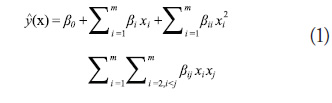
models the response as an explicit function of the independent variables and their interactions. The second order version of this method is given in (1):

where the are the independent variables and the are coefficients that are obtained with least squares regression.

Polynomial regression is a global approximation method that presumes a specific form of the response (linear, quadratic, etc.). Therefore, polynomial regression models are best when the base model is known to have the same behavior as the metamodel. Studies have shown that polynomial regression models perform comparable to kriging models, provided that the base function resembles a linear or quadratic function (Giunta and Watson, 1998; Simpson et al., 1998).

Kriging
Kriging (Sacks et al., 1989) consists of a combination of a known global function plus departures from the base model, as shown in (2):

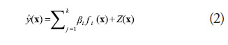
where are unknown coefficients and the are pre-specified functions (usually polynomials). Z(x) provides departures from the underlying function so as to interpolate the training points and is the realization of a stochastic process with a mean of zero, variance of , and nonzero covariance of the form

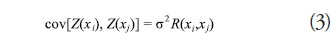
where R is the correlation function which is specified by the user. In this study, a constant term is used for f(x) and a Gaussian curve of the form in (4) is used for the correlation function:

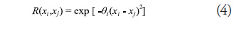
where the terms are unknown correlation parameters that are determined as part of the model fitting process. The automatic determination of the terms makes kriging a particularly easy method to use. Also, contrary to polynomial regression, a krigingmetamodelof this form will always pass through all of the training points and therefore should only be used with deterministic data sets.

Kim et al. (Kim et al., 2009) show that kriging is a superior method when applied to nonlinear, multimodal problems. In particular, kriging outperforms its competitors when the number of independent variables is large. However, it is well documented that kriging is the slowest with regard to build time and prediction time compared with other methods (Jin et al., 2001; Ely and Seepersad, 2009).

Radial Basis Functions
Radial basis functions (Hardy, 1971) use a linear combination of weights and basis functions whose values depend only on their distance from a given center, xi. Typically, a radial basis function metamodel takes the form (5):

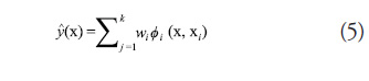
where the is the weight of the basis function, . In this study, a Gaussian basis function of the form in (6) is used to develop the metamodels for testing:

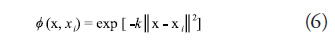
where k is a user specified tuning parameter. Radial basis function metamodels are shown to besuperior in terms of average accuracy and ability to accommodate a large variety of problem types (Jin et al., 1999). However, Kim et al. (Kim et al., 2009) show that prediction error increases significantly for RBF as the number of dimensions increases. This pattern suggests caution must be used when applying RBF to high dimensional problems to ensure that proper tuning parameters are used. RBF is also shown to be moderately more computationally expensive than other methods such as polynomial regression (Fang et al., 2005).

Support Vector Regression
In support vector regression (Vapniket al., 1997), the metamodel takes the form given in (7):

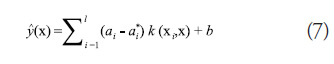
where the a terms are Lagrange multipliers, is a user specified kernel function, and b is the intercept. The a terms are obtained by solving the following dual form optimization problem:

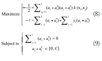
In (8) and (9), l is the number of training points, is a user defined error tolerance, and C is a cost parameter that determines the trade-off between the flatness of the ŷ and the tolerance to deviations larger than . In this study, a Gaussian kernel function of the form in (10) is used to construct the metamodels for testing:

where g is a user specified tuning parameter. Clarke et al. (Clarke et al., 2005) indicate that SVR has the lowest level of average error when applied to a set of 26 linear and non-linear problems when compared to polynomial regression, kriging, RBF, and MARS. SVR has also been shown to be the fastest method in terms of both build time and prediction time (Ely and Seepersad, 2009). An unfortunate drawback of SVR is that accurate models depend heavily on the careful selection of the user defined tuning parameters (Lee and Choi, 2008).

Multivariate Adaptive Regression Splines
Multivariate adaptive regression splines (MARS) (Friedmanl, 1991) involves partitioning the response into separate regions, each represented by their own basis function. In general, the response has the form given in (11):

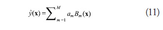
where am are constant coefficients and Bm(x) are basis functions of the form

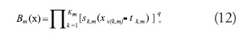
In the Equation (12), is the number of splits in the basis function, take values ±1, are the test point variables, and represent the knot locations of each of the basis functions. The subscript “+” indicates that the term in brackets is zero if the argument is negative. MARS adaptively partitions the design space into sub-regions that have their own regression equations, which enables it to model nonlinear and multimodal responses in high dimensional space.

MARS is shown to predict as well as other methods, but only when a large set of training data is available (Wang et al., 1999, Jin et al., 2001). Using MARS is particularly challenging compared with other methods due to the number of user defined parameters that must be selected. When a large number of basis functions is required to build an accurate model (i.e. nonlinear, multimodal), the build time for MARS can be prohibitively large.

Methods Selected for this Study

Based on the literature reviewed in the previous section, several conclusions can be made about the various metamodeling methods. In general, polynomial regression models can be built and executedvery quickly, even in high dimensions. However, polynomial response surfaces are unable to predict highly non-linear and multimodal functions in multiple dimensions. On the other hand, kriging and radial basis functions are both capable of modeling nonlinear and multimodal functions with higher computation time than polynomial regression. Multivariate adaptive regression splines are capable of modeling multimodal functions in high dimensional space,but often require large training data sets and are computationally expensive to build. Support vector regression, which appears to be the most promising method reviewed here, is shown to be capable of modeling high dimensional multimodal functions accurately with minimal computational expense.

The functions that are modeled in this study range from one to ten dimensions and have modality ranging from one to twenty modes. Polynomial response surfaces are tedious and difficult to construct for multimodal functions due to the exploding number of possible interaction terms that are available for inclusion in the final model. MARS has been shown to be able to model the general behavior of multimodal functions (Jin et al., 1999), but it fails to predict new points accurately at the local maxima and minima. For these reasons, kriging, radial basis functions, and SVR are the primary methods considered in this study.

Test Functions and Experimental Design

To test the ability of polynomial regression, kriging, RBF, and SVR to model functions in high dimensional space, four test functions are used. The first three are generated using a kernel density estimation (KDE) method. The KDE method generates functions in any number of dimensions, containing any number of kernels, where the number of kernels dictates the modality of the resulting surface. The fourth test function is an analytical model of a common engineering system: a two stream counter-flow heat exchanger.

Multidimensional, Multimodal Kernel Based Functions

The need to create test problems of arbitrary dimensionality, D, and arbitrary modality, N, (the number of local maxima or minima) motivates the kernel density estimation (KDE) method. The KDE, also known as a Parzen window (Parzen, 1992), is formulated according to (13) as an average of N kernel functions, K, in product form (Scott, 1992).

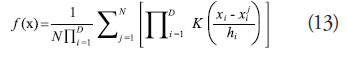
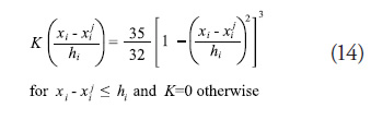
The shape of the KDE is controlled by the kernel function, the kernel centers, , and the smoothing parameters, . For this research, the triweight kernel function (Scott, 1992), shown in Equation (14), was used for its smoothness and for the fact that it is not a Gaussian function which was used as a basis function for some of the metamodeling techniques studied.

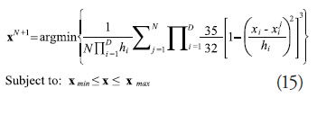
Creating a kernel function of arbitrary dimensionality is straightforward. However, controlling the modality is a bigger challenge for which careful consideration of the kernel centers and smoothing parameters is necessary. For the choice of kernel centers, a certain amount of randomness is desired in the resulting function such that it is unique and its structure is unknown in advance of modeling it. However, a certain amount of control over placement of the kernel centers is needed for creating the requested number of distinct peaks and distributing them throughout the design space. This challenge was met by choosing the kernel centers sequentially such that the next center, , is the minimum of the KDE based on the previous N center points (Equation 15). The first center is chosen from a uniform distribution over the input space.

This method places the next kernel center at the location of minimum density; hence, the resulting sequence of kernel centers fills the space approximately uniformly. The input space is searched for the minimum using multi-start sequential quadratic programming (fmincon in

MATLAB®), stopping if more than one second elapses or less than 1% improvement occurs for 5 consecutive sequential quadratic programming iteration.Although this procedure is not guaranteed to find the global minimum, finding the global minimum is not imperative; we only need to find a point in a low density region. As for the choice of smoothing parameter, setting it too small will result in a surface with spiky peaks at each kernel center, while setting it too large creates humps with maxima that are not necessarily located at the kernel center. However, for the case of the triweight kernel function, one can guarantee an N-modal function by setting the smoothing parameter to 95% of the minimum Euclidean distance between any two kernel centers.

The KDE method is used to create three multimodal functions that are scaled from one through ten dimensions (i.e., one through ten independent variables). In the first scenario, there are N = 2 kernels (modes) regardless of the dimensionality of the problem. In the second scenario, there are N = D kernels, i.e. the number of modes is equal to the number of independent variables. Lastly, in the third scenario, there are N = 2D kernels and the number of modes is always equal to twice the number of independent variables. Posing the problem in this way creates a unique challenge for the metamodeling methods. Specifically, the effect of scaling the number of independent variables can be investigated directly for different levels of modality.

Two Stream Counter-Flow Heat Exchanger

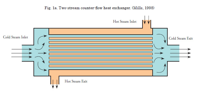
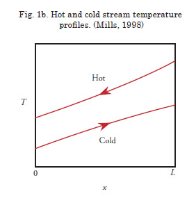
In addition to the functions generated using the KDE method, a two stream, counter-flow shell and tube heat exchanger, such as that used in a shipboard freshwater cooling loop, is used as an example function. A schematic of this type of heat exchanger is shown in Fig. 1a. The heat exchanger features a bundle of conductive tubes inside a cylindrical shell. The hot and cold streams flow in opposite directions resulting in temperature profiles similar to those shown in Fig. 1b. The working fluid in the hot and cold streams is assumed to be fresh liquid water. The temperature dependence of the fluid properties is not ignored, and the outer surface of the shell is assumed to be adiabatic.

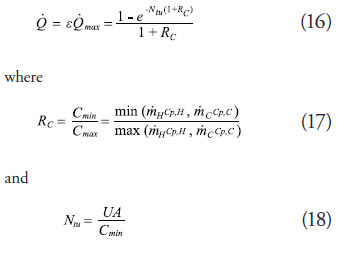
The output of this model is the overall heat transfer rate from the hot stream to the cold stream. This response, given by (16), is obtained by multiplying the maximum theoretical heat transfer rate by the heat exchanger effectiveness

:

In (17), and are the mass flow rates of the hot and cold streams in the heat exchanger, respectively. The and terms refer to the specific heats of the hot and cold streams, respectively. In (18), UA is the overall heat transfer coefficient between the two fluids and is calculated using a combination of conductive and convective heat transfer equations (Mills, 1998). Lastly, the maximum theoretical heat transfer rate is given by (19):

where and are the hot stream and cold stream inlet temperatures, respectively. A thorough explanation and derivation of this heat exchanger model is provided in (Mills, 1998).

Ten independent variables from the above heat exchanger model are selected for this study. The variables and response are listed in Table 1, along with their respective symbols and units. The variables listed in Table 1 are self explanatory with the exception of the flow area ratio. This variable is the ratio of the cross sectional area of the fluid flowing through the shell to the total shell area. It is an indicator of how tightly packed the tubes are within the shell.

To create the one through ten variable test problems that are used in this study, variables are added one

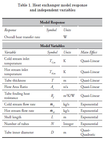
at a time in the order listed in Table 1. The variables whose main effects have the most curvature are added last in an effort to exploit weaknesses of any particular method in high dimensional space.

Experimental Design

Training and Test Point Sampling Strategy
The method for sampling training points from the base model can have a significant effect on the accuracy of the resulting metamodel. In contrast to physical experiments, which are stochastic in nature, deterministic computer models are not subjected to repeated sampling because their predictions typically do not vary unless the input variables change. Therefore, sampling strategies for computer experiments aim to fill the design space as uniformlyas possible (Koehler and Owens, 1996). There are several so-called space filling designs such as Latin hypercube designs (Mckayet al., 1979), Hammersley sequence sampling (Hammersley, 1960), orthogonal arrays (Owen, 1992), and uniform designs (Fang et al., 2000).

Simpson et al. (Simpson et al., 2002) find that uniform designs and Hammersley sequence sampling tend to fill the design space more evenly and provide more accurate results than Latin hypercube designs and orthogonal arrays. They also show that Hammersley sequencing is preferred to uniform designs when large sets of training data can be afforded. In contrast to an expensive computer simulation, all of the test functions used in this paper can be sampled rapidly and large sets of training data are available. Therefore, Hammersley sequence sampling is selected as the method for generating training and test points in this study.

Performance Assessment

In this study, the metamodeling techniques are evaluated based on the number of training points needed to achieve a predetermined error metric. The error metric used is the relative average absolute error (RAAE) and is given by (20):

where is the actual value of the base model at the test points, is the predicted value from the metamodel, n is the number of sample points, and is the standard deviation of the response.

To determine the requirednumber of training points, the quantity of training points is increased continuously until an RAAE value of 0.25 is achieved. The training points are generated with Hammersley sequence sampling. The RAAE is calculated using one hundred test points per variable (100D), which are also generated with a Hammersley sequence.

One issue with this testing strategy is the possibility that some of the training points and test points overlap. For example, in the 1D case, all of the training points will overlap with test points if the number of test points is divisible by the number of test points. Overlapping is to be avoided because testing interpolating methods (kriging and RBF) at the trainingpoints results in zero error. To avoid overlapping in the 1D problem, 101 test points (a prime number) are used. In higher dimensions, test points and training points do not overlap in a Hammersley sequence provided that the number of training points does not equal the number test points.

In addition to the number of sample points necessary to achieve the pre-specified error metric, the computational times required to build each model and to predict the 100D test points are also recorded. All experiments are performed on a 32- bit PC with an Intel Pentium® Dual-Core 2.50 GHz processor with 4.00 GB of RAM.

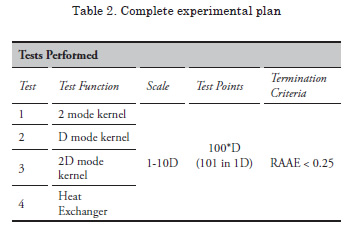
Table 2 includes a summary of the tests to be performed. Metamodels are created in one through ten dimensions for the heat exchanger model and three kernel density estimation functions of varying modality. Performing this task with all three of the metamodeling methods results in a total of 120 tests.

Results and Discussion

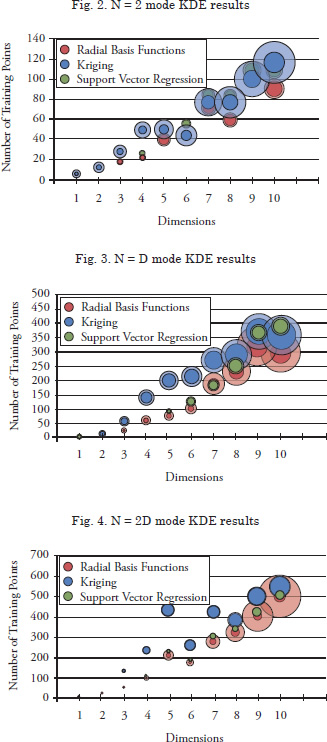
Graphical representations of the results of the study are provided in Figs. 2 to 5. In each figure, the abscissa indicates the dimensionality of each problem, while the ordinate represents the number of training points required to meet the error threshold of RAAE <0.25. The center of each circle represents the number of training points required for the specific dimension and metamodeling method. The size of the solid circles represents the relative training time for each metamodel and the translucent circles represent the relative prediction time for 100D new data points. A complete tabulation of the numerical results is provided in Appendix A.

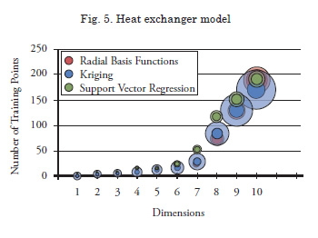
Required Number of Training Points

For all three of the kernel based functions, the general trend is that the required number of training points scales linearly with the number of dimensions. Also, the functions with higher modality require a higher number of training points. In most cases, radial basis function metamodels require the smallest number of training points of the three methods, followed by support vector regression. Kriging metamodels tend to need the highest number of training points of all.

Th e ability of radial basis functions and support vector regression to model the base functions with few training points can be attributed partially to careful selection of user-defi ned tuning parameters. Recall from equations (6) and (10) that the Gaussian basis and kernel functions contain tuning parameters k and g for radial basis functions and support vector regression, respectively. Th e value of these parameters has a signifi cant eff ect on the quality of the resulting metamodel fi t. In this study, these parameters were selected by trial and error until optimal values were obtained. Kriging, on the other hand, has correlation parameters θi that are identifi ed automatically during the fi tting process. Th is automated identifi cation of the correlation parameters is eff ective but requires signifi cant computational expense.

Th e results of the heat exchanger are slightly diff erent than those of the kernel function. Th e required number of training points to model the heat exchanger in most dimensions is very similar for kriging and radial basis functions, with support vector regression needing only slightly more in a few cases. Generally speaking, all methods are able to approximate the heat exchanger model accurately with very few training points when compared to the highly modal and nonlinear function produced using the kernel density estimation method. For the heat exchanger model, the required number of training points increases sharply after 6 dimensions. This result is expected because the variables with the most nonlinear effects are added to the model last, as explained in section 3.2.

Training and Prediction Time

Training and prediction times are represented qualitatively in Figs. 2 – 5 by the size of the solid and translucent circles, respectively. The general trend in all four cases is that the training and prediction times of all methods increase with the number of dimensions. Support vector regression has the smallest training times in all cases. Kriging is slightly slower than radial basis functions when applied to low modality problems in low dimensions. Training times for radial basis functions become very large compared to kriging when applied to high modality, high dimensional problems. The theory behind support vector regression is very computationally efficient (Clarke et al., 2005), and other comparison studies have confirmed its low training times (Ely and Seepersad, 2009). Build times for kriging are expected to be slow because it must perform a nonlinear optimization to obtain the correlation parameters. The slow training times for radial basis functions in highly nonlinear, multidimensional problems stems from the large number of training points required to train an accurate model. During the build process, the RBF method must compute Euclidean distances between adjacent training points. The number of these calculations increases dramatically when the number of dimensions and training points is large.

The manner in which the training times increase with dimensions also varies among the metamodeling methods. The training times for kriging appear to increase linearly with the scale of the problem, but the training times for RBF and SVR begin to increase sharply in the higher dimensional problems. If this trend were extended into very high dimensions, it is possible that the training times for SVR may actually approach or exceed those of kriging.

Support vector regression is also seen to have by far the smallest prediction times of the three methods studied. This trend is also consistent with previous studies (Clarke et al., 2005; Ely and Seepersad, 2009). Kriging has the slowest prediction times of the three methods, being as much as ten times larger than radial basis functions in some cases. Kriging and radial basis function are expected to have large prediction times because the distances between points must be computed during the simulation process (Jin et al., 1999).

Prediction time not only depends on the method used and the scale of the problem, but also on the type of problem being modeled. Even though the number of test points is the same for each respective dimension of each problem, the prediction time increases with the modality of the problem. That is, it takes a given method longer to predict 1000 new points for a more complex problem than it does for a simple one.

Conclusions

In this paper, three types of metamodels— kriging, radial basis functions, and support vector regression—are compared with respect to their speed, accuracy, and required number of training points for test problems of varying complexityand dimensionality. Radial basis functions are found to model and predict the test functions to a predetermined level of global accuracy with the smallest number of training points for most functions. In most cases, kriging metamodels need the highest number of training points of the three methods. Kriging has faster model building times than radial basis functions, but it is slower to predict new data points. Both methods are very slow to train and predict new points when compared to support vector regression.

Metamodel-based optimization has numerous potential applications in the field of marine engineering and ship design. Building ship prototypes and conducting full scale physical experiments are often too expensive or time consuming to be practical in the early stages of the design process, thus driving the need for complex computer models. Using metamodels in place of computationally expensive computer models and simulations can drastically reduce design time and enable ship designers to explore larger regions of the feasible design space.

Acknowledgements

The authors would like to thank the Office of Naval Research (ONR) for supporting this work under the auspices of the Electric Ship Research and Development Consortium. The guidance and experience offered by Dr. Tom Kiehne of Applied Research Laboratories are also gratefully acknowledged.

References

BOX, G. E. P. and K. B. WILSON, 1951, “On the Experimental Attainment of Optimal Conditions,” Journal of the Royal Statistical Society, Vol. 13, pp. 1-45.

CLARKE, S. M., J. H. GRIEBSCH and T. W. SIMPSON, 2005, “Analysis of Support Vector Regression for Approximation of Complex Engineering Analysis,” Journal of Mechanical Design, Vol. 127, pp. 1077-1087.

DIMOPOULOS, G. G., A. V. KOUGIOUFAS and C. A. FRANGOPOULOS, 2008, “Synthesis, Design, and Operation Optimization of a Marine Energy System,” Energy, Vol. 33, pp. 180-188.

ELY, G. R. and C. C. SEEPERSAD, 2009, "A Comparative Study of Metamodeling Techniques for Predictive Process Control of Welding Applications," ASME International Manufacturing Science and Engineering Conference, West Lafayette, Indiana, USA, Paper Number MESC2009-84189.

FANG, H., M. RAIS-ROHANI, Z. LIU and M. F. HORSTMEYER, 2005, “A Comparative Study of Metamodeling Methods for Multiobjective Crashworthiness Optimization,” Computers and Structures, Vol. 83, pp. 2121-2136.

FANG, K. T., D. K. J. LIN, P. WINKER and Y. ZHANG, 2000, “Uniform Design: Theory and Applications,” Technometrics, Vol. 42, No. 3, pp. 237-248.

FRIEDMAN, J. H., 1991, “Multivariate Adaptive Regression Splines,” The Annals of Statistics, Vol. 19, No. 1, pp. 1-67.

GIUNTA, A. and L. T. WATSON, 1998, "A Comparison of Approximation Modeling Techniques: Polynomial Versus Interpolating Models," 7th AIAA/USAF/ISSMO Symposium on Multidisciplinary Analysis & Optimization, St. Louis, MO, AIAA, Vol. 1, pp.392-404. AIAA-98-4758.

HAMMERSLEY, J. M., 1960, “Monte Carlo Methods for Solving Multivariable Problems,” Annals of the New York Academy of Sciences, Vol. 86, pp. 844-874.

HARDY, R. L., 1971, “Multiquadric Equations of Topology and Other Irregular Surfaces,” Journal of Geophysical Research, Vol. 76, No. 8, pp. 1905-1915.

HAYKIN, S., 1999, Neural Networks: A Comprehensive Foundation, Prentice Hall, Upper Saddle River, N.J.

JIN, R., W. CHEN and T. W. SIMPSON, 2001, “Comparative Studies of Metamodeling Techniques Under Multiple Modeling Criteria,” Structural and Multidisciplinary Optimization, Vol. 23, pp. 1-13.

KIM, B.-S., Y.-B. LEE and D.-H. CHOI, 2009, “Comparison Study on the Accuracy of Metamodeling Technique for Non-Convex Functions,” Journal of Mechanical Science and Technology, Vol. 23, pp. 1175-1181.

KOEHLER, J. R. and A. B. OWENS, 1996, "Computer Experiments," Handbook of Statistics, Elsevier Science, New York, Vol. 13, pp. 261-308.

LEE, Y., S. OH and D.-H. CHOI, 2008, “Design Optimization Using Support Vector Regression,” Journal of Mechanical Science and Technology, Vol. 22, pp. 213-220.

MCKAY, M. D., R. J. BECKMAN and W. J. CONOVER, 1979, “A Comparison of Three Methods for Selecting Values of Input Variables in the Analysis of Output from a Computer Code,” Technometrics, Vol. 21, No. 2, pp. 239-245.

MILLS, A. F., 1998, Heat Transfer, Prentice Hall, Upper Saddle River, NJ.

OWEN, A. B., 1992, “Orthogonal Arrays for Computer Experiments, Integration, and Visualization,” Statistica Sinica, Vol. 2, pp. 439-452.

PARZEN, E., 1962, “On Estimation of a Probability Density Function and Mode,” The Annals of Mathematical Statistics, Vol. 33, No. 3, pp. 1065-1076.

PERCIVAL, S., D.HENDRIX and F. NOBLESSE, 2001, “Hydrodynamic Optimization of Ship Hull forms,” Applied Ocean Research, Vol. 23, pp. 337-355.

PERI, D., M. ROSSETTI and E. F. CAMPANA, 2001, “Design Optimization of Ship Hulls via CFD Techniques,” Journal of Ship Research, Vol. 45, No. 2, pp. 140-149.

RACINE, B. J. and E. G. PATERSON, 2005, "CFD-Based Method for Simulation of Marine- Vehicle Maneuvering," 35th AIAA Fluid Dynamics Conference and Exhibit, Toronto, Ontario Canada.

SACKS, J., S. B. SCHILLER and W. J. WELCH, 1989, “Designs for Computer Experiments,” Technometrics, Vol. 31, No. 1, pp. 41-47.

SCOTT, D. W., 1992, Multivariate Density Estimation, John Wiley & Sons, Inc., New York.

SIMPSON, T., L. DENNIS and W. CHEN, 2002, “Sampling Strategies for Computer Experiments: Design and Analysis,” International Journal of Reliability and Application, Vol. 2, No. 3, pp. 209-240.

SIMPSON, T. W., T. M. MAUERY, J. J. KORTE and F. MISTREE, 1998, “Comparison of Response Surface and Kriging Models for Multidisciplinary Design Optimization,” 7th AIAA/USAF/NASA/ISSMO Symposium on Multidisciplinary Analysis and Optimization, Vol. 1, pp. 381-391.

VAPNIK, V., S. GOLOWICH and A. SMOLA, 1997, “Support Vector Method for Function Approximation, Regression Estimation, and Signal Processing,” Advances in Neural Information Processing Systems, Vol. 9, pp. 281-287.

WANG, X., Y. LIU and E. K. ANTONSSON, 1999, "Fitting Functions to Data in High Dimensionsal Design Space," ASME Design Engineering Technical Conferences, Las Vegas, NV, Paper Number DETC99/DAC- 8622.

WATANABE, T., T. KAWAMURA, Y. TAKEKOSHI, M. MAEDA and S. H. RHEE, 2003, "Simulation of Steady and Unsteady Cavitation on a Marine Propeller Using a RANS CFD Code," Fifth International Symposium on Cavitation, Osaka, Japan.