Creating Bathymetric Maps Using AUVs in the Magdalena River

Dr. Monique Chyba¹
John Rader²
Michael Andoinian³

Abstract

The goal is to develop a guidance and navigation algorithm for an AUV to perform high resolution scanning of the constantly changing river bed of the Magdalena River, the main river of Colombia, from the river mouth to a distance of 10 Km upriver, which is considered to be the riskiest section to navigate. Using geometric control we design the required thrust for an under-actuated autonomous underwater vehicle to realize the desired mission.

Key words: River Survey, Autonomous Underwater Vehicle

Resumen

El objetivo es desarrollar un algoritmo de orientación y navegación para un AUV (Autonomous Underwater Vehicle) para realizar el escaneado de alta resolución del cambiante lecho del río Magdalena, principal río de Colombia, desde su desembocadura hasta una distancia de 10 Km río arriba, que se considera la sección de mayor riesgo para navegar. Usando control geométrico se diseñó el empuje necesario para un vehículo submarino autónomo subactuado para realizar la misión deseada.

Palabras claves: Vehículo submarino autónomo

Date received: May 20th, 2010. - Fecha de recepción: 20 de Mayo de 2010.
Date Accepted: July 6, 2010. - Fecha de aceptación: 6 de Julio de 2010.

________________________

¹ University of Hawaii at Manoa, Honolulu, HI. e-mail: mchyba@math.hawaii.edu
² University of Hawaii at Manoa, Honolulu, HI. e-mail: jrader@hawaii.edu
³ University of Hawaii at Manoa, Honolulu, HI. e-mail: andonian@hawaii.edu

............................................................................................................................................................

Introduction

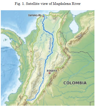
One of the primary initiatives of the country of Colombia is the constant surveillance of the everchanging waterways used as shipping lanes. The Magdalena River, the main river of Colombia to which 25% of the Growth Domestic Product (GDP) can be directly associated, is a major shipping lane, as the river penetrates deep into the heart of the country. From southwestern Colombia, it fl ows approximately 1,000 miles (1,600 km) northward to the Caribbean Sea—past Neiva, Girardot, and the port of Barranquilla (see Fig. 1). Navigable for most of its length, the Magdalena is a major freight artery. For centuries, it has provided a main route to the interior, and its inland waterways transport approximately 3.8 million metric tons of freight and more than 5.5 million passengers annually. Also, said waterways serve as the only means of transportation in 60% of the country due to the lack of navigable roadways.

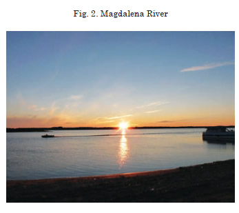
The Magdalena waterway is one of the most important waterways in the country, accounting for 45 percent of the 2007 cargo movement, Ministry of Transportation (2008). Major products shipped through the Magdalena River are petrochemicals, machinery, cattle, cement, fertilizers, and wood. Due to the river’s continuous change, shipping on the river requires trans-shipments and does not operate at full capacity due to lack of investments (totaling 1% of the yearly GDP) in dredging, channel improvements, and protective levies. From Barranquilla to Capulco (about 310 miles), the river is navigable with a depth of only 6 feet allowing night navigation with satellite navigation systems (see Fig. 2). However, due to the impact of many variables, the river must be weekly monitored for depth, currents, and velocity, primarily depth, and especially during the rainy season due to the higher concentration of silt, debris, and/or particulates that can accumulate.

The main way that the monitoring has been done is manually; that is, physical measurements are made by observers on boats. Considering that this is done weekly and over large areas, it is very ineffi cient and time consuming. We propose a new way of river monitoring by using Autonomous Underwater Vehicles (AUVs) that will, using the most recent map prior to implementing the AUVs, run specifi c missions in order to obtain the necessary data to create accurate maps for river navigation. Th rough a variety of missions the AUV will determine actual depths and produce precise maps of said depths, as well as determine river velocities and directions such that precision maps can be produced without requiring physical measurements by observers.

Clearly, this work is still at a very theoretical stage, many additional constraints will have to be taken into account to make it implementable on a real test-bed vehicle. But it provides a fi rst step into that direction.

Mision

The goal is to develop a guidance and navigation algorithm for an AUV to perform high resolution scanning of the constantly changing river bed of the Magdalena River from the river mouth to a distance of 10km upriver, which is considered to be the riskiest section to navigate.

We choose to analyze this section since it is considered to be a priority shipping lane and to prevent future shipping failures/groundings. We plan the trajectories of the AUV according to the most recently produced manual bathymetry map. The AUV will be released upstream, dive to a safe depth to avoid surface traffic, will ride the current until it reaches an area of interest, and then will scan, at a depth of around 6-10 meters, considered a navigable depth for all river traffic, in and around these sections that are determined to be deepest from the previous bathymetry map. The missions will include scanning deeper sections of the river to determine exact sizes of these navigable areas and river bathymetry, as well as monitoring river velocity at depths and determining local current directions at cross-sections that are evenly spaced along the river’s length. Upon completion of a scanning mission, it will migrate to the next section of interest and will continue so forth until all areas of interest are covered, and/or the battery dies, and/or battery weakens so that the AUV cannot counteract the force of the current, at which point it will migrate downstream until reaching the ocean. Once there, it will surface and send the collected data via satellite as well as a GPS signal so that the AUV can be recovered and it can be recharged and re-released upstream to collect more data. The data will then be used to create a highly, accurate bottom profile and, accordingly, a navigable map that can be used by boat captains. The use of an AUV will significantly minimize the number of persons required previously, as well as the amount of time to collect the bathymetry data. In fact, only one skilled person with access to a ocean- and river-faring boat (with a small crane) and a vehicle (with a lift) is required to perform this task. Also, the data can be collected more regularly than the current weekly collection, thus providing boat captains with daily updates to bathymetry changes.

Although this initially may seem redundant to any captain, if a grounding/sinking occurs, it will be highly apparent to anyone involved in the shipping process (particularly the owners of the boat and cargo) how valuable having accurate, dailyproduced bathymetry maps truly is.

Vehicle Design

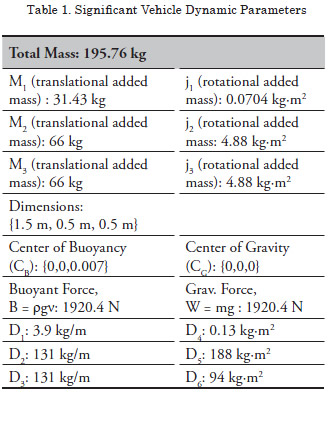
The chosen design of the vehicle has been determined by several factors. First, the mission itself imposes specific characteristics to the vehicle such as its shape and actuation mode. An equally critical component in vehicle’s design is the controllability capabilities that will be available to complete the mission. Those are determined from several criteria as it is explained below. Our approach here differs from our previous work in which the controllability of the vehicle was a consequence of the vehicle’s design. Typically, for missions involving river and long-transect ocean surveys, torpedo-shaped AUVs are used, Fig. 3. The dimensions and characteristics of the vehicle are given in Table 1.

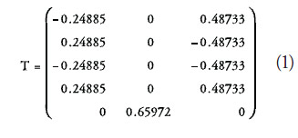
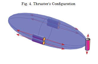
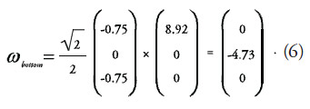
Our vehicle model is based loosely on the Starbug AUV and a REMUS 100 vehicle, which both have similar dimensions. Based on the empirical data of REMUS and the Starbug, we assume the vehicle here has a maximum speed of 1.5 m/s. Th is is not preposterous by any means, as we've added two additional thrusters, Fig. 4, which would logically have the same capabilities as those on the other two AUVs, to account for the size diff erence. Added mass terms and drag coeffi cients are assumed to be similar to those of the REMUS. Such parameters can be found in Dunababin (2005) and Prestrero (2001). Our choice of actuation using thrusters comes from the fact that the AUV will be functioning in a river environment with currents. Gliders are extremely popular and effi cient in open ocean, see Slocum, Remus, and Fleet, however they do not have the capability to respond quickly to abrupt changes in the environment and, therefore, are not suitable for river surveys. Our goal here is to produce a thruster confi guration using a minimal number of thrusters but allowing maximum fl exibility and controllability. To this end, we refer to previous work on kinematic controllability Smith (2009a). In Smith (2009a), it has been shown that any combination of one translation and two rotational degrees of freedom provides a system that is kinematically controllable. More precisely, an underwater vehicle with direct control in either one of the translation motion (surge, sway, heave) as well as two rotational motions (roll, pitch, sway) can reach any confi guration by the use of integral curves of the decoupling vector fi elds (see section on Control Design) corresponding to this actuation confi guration scenario. Our choices of the directly controllable degrees of freedom are surge, yaw, and pitch. Th is is motivated by the river environment in which the vehicle interacts. From our thruster confi guration, we note that our vehicle begins (and will remain) under-actuated. Th us, the only permissible degrees of freedom available to us correspond to surge, pitch, and yaw motions. Moreover, the four thrusters contributing to surge and yaw give us a bit of a leeway in the event of thruster failure. If a thruster on either side were lost, we would retain controllability over surge and yaw, albeit maximum thruster power is no longer available. Given our thruster confi guration, it is necessary to have a linear transformation which takes the geometric controls in the available three degrees of freedom from the body-frame and yields the needed controls for each thruster to accomplish said motion. Th is corresponds to the matrix given below,

Moreover, we will set the maximum force output of any thruster to be 2.25 Newtons (N). Th us, the maximum force of the four thrusters contributing to surge and yaw is 9 N. Th is means the front, vertical thruster has a maximum torque of 6.75 Newton-meters (Nm).

Control Design

Th e calculations of the dynamic controls to achieve the AUV mission are done in several steps. First, based on our choice of the thruster's confi guration, we determine a path in the confi guration space for our vehicle to survey pre-determined areas of the river. This is done through a concatenation of kinematic motions. Second, using an inverse kinematic procedure, we compute the corresponding controls for the dynamic system. The inverse kinematic procedure does not allow for the incorporation of restoring forces and moments nor for the current of the water. A third step is necessary to compensate for the fact that our vehicle is not neutrally buoyant and that the center of gravity and buoyancy do not coincide. And finally the current of the river is taken into account in the calculations of the dynamic controls. Once all the steps have been completed, the vehicle will follow the prescribed path in the configuration space using the calculated thrust.

Kinematic motions

We present a typical motion in the configuration space (position + orientation) to realize the AUV's mission. As mentioned before, the degrees of freedom that are directly controlled are surge (a natural choice in the environment as it is aligned with the river current) coupled with yaw and pitch. This pair of angular degrees of freedom is arbitrary in choice (we could have opted for a combination of yaw/roll or roll/pitch to achieve motion in all six degrees), but this choice is more relevant in reference to the kinematic paths designed for the AUV. We chose the yaw and pitch angles specifically so that the motions in the induced directions (sway and heave) could be facilitated by the force of the current to conserve the AUV's energy, which is important in considering how the AUV would survey the specific region of choice, in this case an arbitrary rectangular region. To be able to apply our theory to compute the dynamic controls, we must insure that the kinematic paths can be obtained as integral curves of decoupling vector fields for the given thruster's configuration. We refer the reader to Smith (2009a) for more information about the theoretical calculations of our strategy. In short, the idea is that the decoupling vector fields are of kinematic reduction of rank one, and their integral curves represent motion in the configuration space that are called kinematic motions. The important feature of kinematic motions is that they are feasible by the actual vehicle, or in other words it means that, through an inverse kinematic procedure, we can determine the power output that the thrusters must provide to follow the motion exactly. We chose paths such that the long axis of the vehicle is aligned parallel to the river current (when in the standard orientation) as often as possible as to minimize drag forces caused by the current (to be as hydrodynamic as possible), and when not in standard orientation, the vehicle utilizes the current. Once the vehicle reached an area of interest, it performs transects perpendicular to the river current, as opposed to parallel transects. The reason for this choice comes from the fact that the total amount of energy required for parallel transects would be much greater than the total energy required for perpendicular transects. Indeed, during a pair of parallel transects the vehicle initially uses zero energy since it is riding the current downstream, but after moving to the next parallel transect, which is now oriented upstream, the vehicle has to fight the current to reach the original location and requires large amounts of energy, not to mention the energy needed by the AUV to move from one transect to the next. However, in the perpendicular transects, the vehicle uses a constant amount of energy only to balance the drag forces and maintain its orientation, and moving to the next perpendicular transect requires zero energy as the vehicle rides the current downstream to it. Hence it is more efficient as it utilizes more of the available energy from the environment.

Dynamic controls

We refer the reader to Bullo-Lewis (2004), and Smith (2009b), for a complete treatment on the inverse procedure to obtain the dynamic controls. It is out of the scope of this paper to repeat those derivations here. It has to be noted, however, that the inverse procedure provide the dynamic controls without taking into account the restoring and potential forces as well as the river current. How to compensate for the restoring and potential forces can be found for instance in Andonian et al. (2010). We are explicit in this paper how to adjust the controls to take into account the river’s current, see section on Simulations.

Simulations

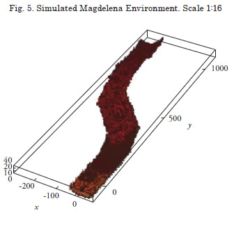
In this section, we bring life to the theory by considering a simulation using the vehicle and mission plan described previously. Th e environment we are simulating, the Magdalena River in Fig. 5, is particularly interesting due to the fact we must now account for the river's fl ow. We assume the current of the river has a constant velocity of 2 m/s throughout depths of 0-5 meters, a constant velocity of 1.5 m/s throughout depths of 5-7 meters, and a constant velocity of 1 m/s throughout depths of 7-12 meters. Th ese values are based on data from the Laboratorio Las Flores from Cormagdalena- Uninorte in Barrancabermeja, Colombia. As usual, the positive vertical axis of the inertial frame is in the direction of gravity.

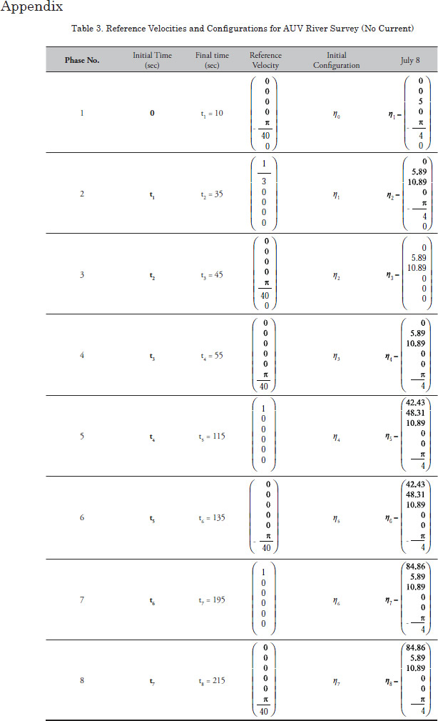
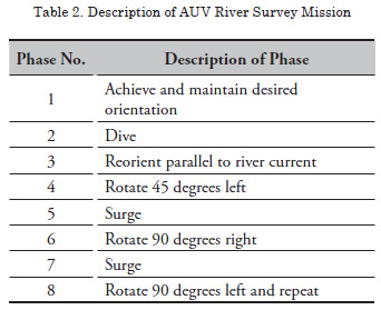
In Table 2, we give a full reference for each of the eight phases of the mission. The configuration and time for each phase can be found in Table 3 of the Appendix.

Let us now begin the simulation of the mission. Th e vehicle will be initially deployed upstream and travel downstream until it reaches a desirable section. We assume the AUV is oriented to be “facing” downstream and assume it is fi ve meters below the surface. Th e symbol, ƞ, will represent a vector whose fi rst three components refer to the vehicle's position and the last three components to orientation, in terms of Euler angles, in the inertial frame. Our initial confi guration will be where the

vehicle begins its mission. As such, the origin of the inertial frame will be taken at the surface of the water before the exploration mission begins. Th us, the initial confi guration is,

Note, the velocity of the river's current exceeds the vehicle's maximum speed; thus, if we do not compensate for this speed diff erence, we will obviously drift past the target. More on this point will be discussed later. For the fi rst phase, the vehicle pitches 45 degrees towards the riverbed and maintains this angle. Since CG ≠ CB, there are righting moments we must consider. In general for our system, they are given by,

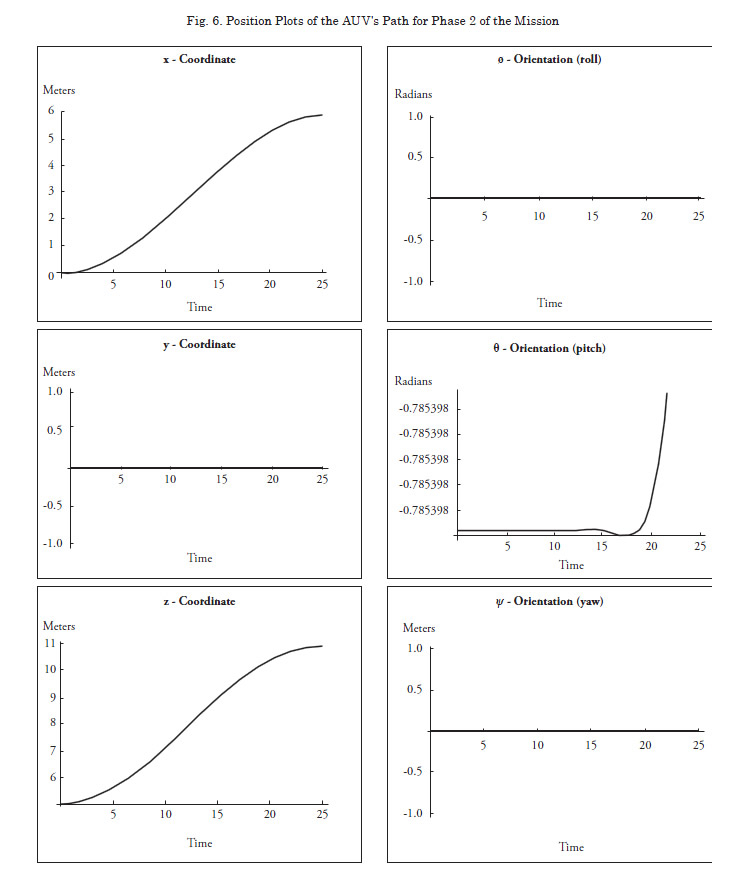
where B is the buoyancy force and is the z-coordinate for the location of the center of buoyancy of the vehicle. For the second phase, the vehicle descends at this 45 degree angle for 25 seconds until it reaches the 10.89 meters in depth. Fig. 7 gives the six plots for the confi gurations throughout this phase, beginning at and ending at .

At this point, we are in an area of the river where the vehicle's maximum speed exceeds the river's current. The third phase of the mission involves the vehicle reorienting itself to become parallel with the river's surface again. During the fourth phase, the vehicle must counteract the river's current. The vehicle then proceeds to survey the riverbed as described in phases 5 – 9 in Table 2.

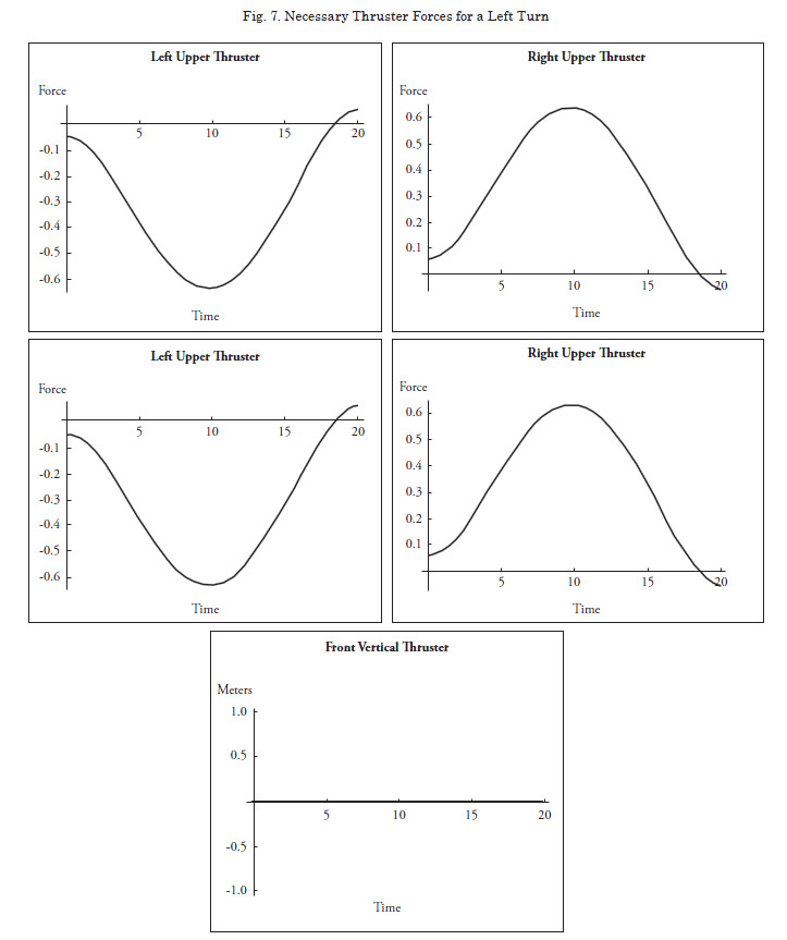
The final phase has the vehicle reorienting itself parallel to the current yet again. Fig. 8 shows plots of the necessary forces for each of the thrusters in order to turn 45 degrees to the left. Due do the redundancy in our control strategy, note the negative values for each of these thruster force plots corresponds to the necessary forces to turn the vehicle 45 degrees to the right. The vehicle must then repeat phases 4-8 until enough data is collected to complete the mission objective. We now move on to the second half of the simulation discussion and adjust our controls to account for the river current.

Let us define our controls to be where i refer to the mission phase and j is the jth component of the configuration. In addition, we assume these already have the necessary restoring forces included. Similarly, we will define to be the adjusted controls that compensate for the river current. Th ese controls correspond to the bodyfi xed frame, geometric controls. Recall that the maximum forward thrust of the vehicle is 9 N and the maximum torque is 6.75 Nm.

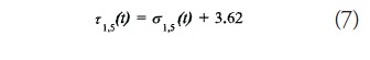
Now turning our focus to phase one of the mission plan, we must determine the required control’s adjustment in order to maintain our pitch of 45 degrees pointing down towards the river bed given the river’s current. Th eoretically, if the vehicle is in a horizontal orientation, and was to maintain a velocity of 2 m/s, it would need to exert 15.74 Newtons of force; this force would keep the vehicle stationary in the river and so we will assume 15.74 N is the amount of force exerted on the vehicle by the river's current at 2 m/s. With the vehicle pitched as it is in phase one, the current will induce a moment on the vehicle. Assuming the vehicle is a point mass at the center of gravity, we utilize classical physics to calculate the torque the vehicle would need to exert to maintain its pitch.

Th us, the “lever arm” is the distance from the center of gravity to the vertically mounted thruster, which is 0.75 meters. Fig. 8 shows a side profi le of the vehicle and the signifi cant parameters. Since we are only concerned with our pitch angle, all other controls are zero. Using Fig. 8 as a basis, we fi nd the torque acting on the portion of the vehicle above the dotted line is given by

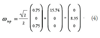
Thus, there is a torque of 8.35 Nm that must be considered in the controls. Let us remark again that the vehicle is assumed to be experiencing a constant force above the dotted line and below the dotted line. Th is allows us to simply sum all the torques to fi nd what kind of moment we must counteract. Th is gives us a new control

where the additional torque is added to the original controls. We added this torque due to the fact that the current at 2 m/s is righting our pitching motion. However, the vehicle is also experiencing a force below the dotted line. Th is torque turns out to be

which ultimately (by summing the torques) gives us the control we need to maintain the pitch,

Note, we are within our bounds.

For phase 2, the situation gets more complicated. As the vehicle descends into the river, the velocity of the current acting on the vehicle changes. For these controls, we will assume the vehicle must counteract the most powerful forces to not drift backwards. Th us, from Fig. 7 we can assert the vehicle does not completely pass through the 2 m/s current until t = 15.7s and does not pass through the 1.5 m/s current until t = 22s. Th e force needed to counteract the 2 m/s current during the dive is 22.19N (note that this force is higher than 15.74N due to the fact that the vehicle is maintaining a pitch), and to counteract the 1.5 m/s current is 12.58N. However, these are outside the maximum thruster output of the vehicle, so we will drift downstream. Then, at time t = 22s, the vehicle completely passes into the region of the river where the current velocity is 1 m/s. To remain stationary at this pitched angle, the vehicle must apply 5.7N of forward thrust. However, once the vehicle completely passes into 1 m/s flow range, there are no longer any moments to account for. Our controls now become

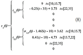
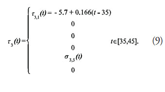
to complete phase two. Now, we look to discover the necessary controls to complete phase 3. We will assume it takes ten seconds still to reorient the vehicle. However, we wish to remain stationary for an additional 30 seconds. Again, we need not worry about the force of the current causing a moment on the AUV, as the sum of the torques is zero. As such, the only control we are searching for corresponds to surge; the sway control on the other hand remains the same as before without the river current. The initial body-frame forward thrust will still be 5.7 N to not surge, dive, or drift and will end with a thrust force of 4.04 N, which is the force we need to remain stationary with the vehicle parallel to the current flow. Thus, the new controls running from t =35s to t = 45 s are

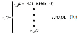
Finally, we compute the necessary controls for phases 4, 5, and 6. Due to the redundancy of this control strategy, we need not compute the remaining controls, as they will be the same but simply allocated differently to the thrusters. For phase four, we must perform a yaw maneuver to turn left. Since we begin to experience a moment as soon as we begin the turn left, we will assume we must compensate for this torque the entire time. This torque is the same as before 2.14 Nm, but in a different plane. The same can be said about the compensating thruster force to keep the vehicle from drifting in the y-plane; this must be 4.04 N initially and 5.7 N when the vehicle has rotated 45 degrees to the left. Assuming the time it takes the vehicle to rotate remains ten seconds, beginning at t = 45s and ending at t = 55s, our controls become

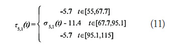
Note that there are no moments we must compensate for. This is because the sum of the torques acting on the vehicle at any angle for parallel with the river's flow will again be zero. For phase five, we adjust our controls only slightly to compensate for the current,

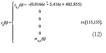
And finally, we wish to execute phase six; the necessary controls are

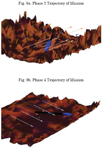
Figures 9a and 9b represent simulations in the river environment of Phases 2 and 4, respectively, of the mission. In the fi gures, the dashed orange vectors correspond to the river current velocity at 2.0 m/s, the dotted blue vectors correspond to the river current velocity at 1.5 m/s, and the solid white vectors correspond to the river current velocity at 1.0 m/s. Also, the vehicle is magnifi ed by a factor of 8 for visualization purposes only.

References

ANDONIAN, M., CAZZARO, L., INVERNIZZI, L, and CHYBA, M. Geometric Control for Autonomous Underwater Vehicles: Overcoming a Th ruster Failure.IEEE Conference on Decisions and Control. Atlanta, GA. 2010.

BULLO, F. and LEWIS, A. Geometric Control of Mechanical Systems, Texts in Applied Mathematics, Springer, ISBN 0-387-22195-6, 2004.

DUNBABIN, M., ROBERTS, J., USHER, K., WINSTANLEY, G., and CORKE, P. A Hybrid AUV Design for Shallow Water Reef Navigation. IEEE.Proceedings of the 2005 IEEE International Conference on Robotics and Automation. Barcelona, Spain. 2005.

FLEET. http://marine.reutgers.edu/cool/auvs/ MINISTRY OF TRANSPORTATION, Ofi cina Asesora de Planeacion, Grupo de Planifi cacion Sectorial,Diagnósticodel Sector Transporte, 2008. http://www.mintransporte.gov.co/ Servicios/Estadisticas/home.htm

PRESTERO, T. Verifi cation of a Six-Degree of Freedom Simulation Model for the REMUS Autonomous Underwater Vehicle. Master’s thesis. MassachusettsInstitute of Technology and Woods Hole Oceanographic Institution, Joint Program in Applied Ocean Science and Engineering. 2001.

REMUS. http://www.hydroidinc.com/ SLOCUM. http://www.webbresearch.com/ slocumglider.aspx

SMITH, R. and CHYBA, M. Trajectory Design for Autonomous Underwater Vehicle for Basin Exploration. 8th International Conference on Computer Applications and Information Technology in the Maritime Industries (COMPIT), Budapest 2009

SMITH, R., CHYBA, M., WILKENS, G., and CATONE, C. A Geometrical Approach to the Motion Planning Problem for a Submerged Rigid Body. International Journal of Control, Vol. 82/9, pp. 1641 -1656, 2009.