SPH Boundary Deficiency Correction for Improved Boundary Conditions at Deformable Surfaces

Van Jones¹
Qing Yang²
Leigh McCue-Weil³

Abstract

Smoothed particle hydrodynamics (SPH) is a meshless, Lagrangian CFD method. SPH often utilizes static virtual particles to correct for integral deficiencies that occur near boundaries. These virtual particles, while useful in most cases, can be difficult to implement for objects which experience large deformations. As an alternative to virtual particles, a repulsive force algorithm is presented which loosely emulates the presence of virtual particles in the SPH momentum equation.

Key words: Smoothed Particle Hydrodynamics, SPH, SPH Boundary Condition.

Resumen

La Hidrodinámica de Partículas Suavizadas (Smoothed Particle Hydrodynamics, SPH) es un método CFD Lagrangiano sin malla (Mecánica de Fluidos Computacional, CFD). El método SPH frecuentemente utiliza partículas estáticas virtuales para corregir las deficiencias integrales que ocurren cerca de las fronteras. Estas partículas virtuales, aunque son útiles en la mayoría de los casos, pueden ser difíciles de implementar para objetos que experimentan grandes deformaciones. Como alternativa a las partículas virtuales, se presenta un algoritmo de fuerza repulsiva que emula indirectamente la presencia de las partículas virtuales en la ecuación de momento del método SPH.

Palabras claves: Hidrodinámica de Partículas Suavizadas, Condiciones de frontera de SPH.

Date received: May 20th, 2010. - Fecha de recepción: 20 de Mayo de 2010.
Date Accepted: July 6, 2010. - Fecha de aceptación: 6 de Julio de 2010.

________________________

¹ Virginia Tech. e-mail: cerchio@vt.edu
² Virginia Tech. e-mail: royyang@vt.edu
³ Virginia Tech. e-mail: mccue@vt.edu

............................................................................................................................................................

Overview of Smoothed Particle Hydrodynamics

Smoothed particle hydrodynamics was fi rst developed for applications in astrodynamics [1][2]. SPH was later adapted to fl uid dynamics due to its ability to effi ciently simulate complex free surface fl ows. It is based on the ability of a kernel function to approximate a fi eld value at a point by integrating over surrounding fi eld values. A kernel function is a fi nite area approximation of the Dirac delta function. The SPH approximation can be seen by fi rst considering the integration result of the product of a fi eld and the Dirac delta function (Eqn 1a). Th is integration exactly yields the fi eld value at the location of the Dirac delta function. By replacing the discontinuous Dirac delta with a kernel function possessing similar properties (but defi ned over a fi nite area) a useful approximation of fi eld functions can be obtained (Eqn 1b). This formula can then be discretized to obtain an equation applicable to Lagrangian particle dynamics (Eqn 1c). In the discretization, is the value of the kernel function between a subject particle (i) and an influencing particle (j) with as the area or volume associated with the infl uencing particle [8].

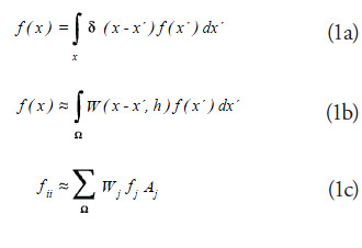
Th e integration limits for Eqn 1a can be infi nite with identical results. However, because the integration product is zero everywhere except at x' = x, the integration limits can be reduced to encompass only the point x. Similarly, most kernel functions with compact support domain are defi ned as zero beyond a set radius. It follows that the integration/summation region for Eqns 1b and 1c need only encompass the region in which the kernel function is defi ned to be non-zero.

A classic kernel function, described by Monaghan and Lattanzio, is the Cubic-spline function (Fig. 1) [12]

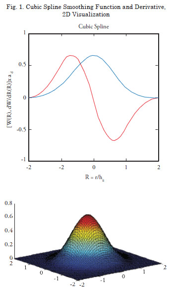
The Cubic-spline kernel function is defi ned as nonzero for all r < 2h (where h is a scaling parameter typically based on particle mass). It follows that the integration domain Ω of equation 1b is the region within a radius of 2h of the point x. Similarly, for equation 1c the support domain particles (Ω) consist of all particles within 2h of the subject particle i as illustrated in Fig. 2.

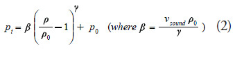
Th e SPH method can be applied to fl uid dynamics in a number of ways. A common technique to adapt SPH to fl uid dynamics is Weakly Compressible Smoothed Particle Hydrodynamics (WCSPH). In WCSPH, fluids typically considered nearly incompressible are allowed a small degree of compressibility. Th is yields a fi nite speed of sound for the fluid and changes the characteristic of the governing equations to allow for uncoupled solving of particle properties. Particle pressures are derived from an equation of state. The parameters of the equation of state determine the numerical speed of sound in that medium. The Tait Equation (Eqn 2) is a commonly used equation of state for water simulations [13].

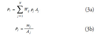
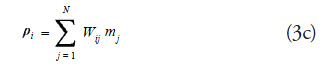
Two common methods exist to calculate SPH particle density, these are the summation and continuity density formulations. The summation density formulation directly determines density by summing the kernel-weighted densities of all support domain particles (Eqn 3a). Substituting the definition of density (Eqn 3b) into Eqn 3a yields Eqn 3c [8] and tranforms the formula into a mass summation over an implied volume (the kernel function has units of inverse volume).

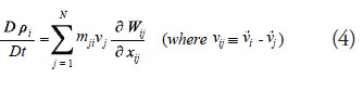
The continuity density formulation instead calculates the velocity divergence for each particle. Because the velocity divergence of a fluid is equivalent to the time rate-of-change of density this value can be integrated over time to obtain density change. The corresponding particle discretized formula for the continuity density formulation is shown in equation 4 [8].

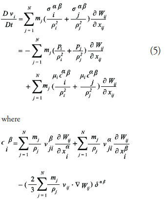
Particle acceleration is determined from the stress tensor for each particle . The stress tensor can be separated into translational (pressure) and viscous shear stresses. Shear stress can be approximated as the product of fluid's dynamic viscosity (μ) and strain rate tensor . For inviscid cases (μ=0), the particle discretized momentum equation reduces to a simple pressureforce summation. Equation 5 shows the particle discretized SPH momentum equation [8].

SPH Boundary Behavior

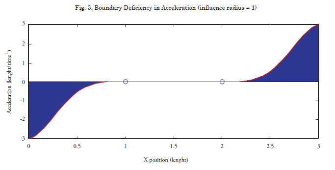
Assuming uniformly distributed particles in an unbounded region, the SPH particle discretized governing equations approach the Navier Stokes governing equations as smoothing length approaches zero. The unbounded assumption is required to satisfy that fluid field values exist at all points within a particle's support domain. When a particle's support domain has an insufficient number of particles to adequately approximate the fluid field values within its support radius it is said to be integral or boundary deficient. One way in which this can occur is if particle smoothing radius is set to a small value such that very few particles fall within a support radius, in this case the SPH governing equations will yield poor approximations of field functions. Because of this smoothing radius is typically empirically related to particle mass and density such that an acceptable influence radius is maintained. A second more complicated manner in which integral deficiency can occur is observable when a particle is within close proximity to a fluid boundary. This situation is shown in Figure 3, which plots particle acceleration of a finite 1D constant pressure fluid. While there exists no pressure gradient in the fluid, nearboundary particles exhibit a non-zero acceleration or boundary deficiency in acceleration.

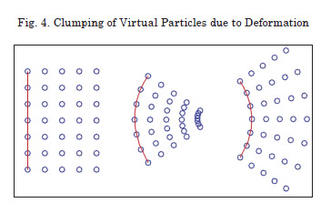
This behavior is desirable at free surfaces for singlephase simulations as the boundary deficiency behaves identically to a zero gauge pressure fluid. However, boundary deficiency leads to difficulties at fluid-object boundaries. Relatively robust boundary conditions can be created by using repulsion forces based on spatial proximity (see [3][4][5]). However, because of the lack of a pressure term to correct for boundary deficiency, proximity-based repulsion boundaries tend to yield a nonphysical varying fluid particle to wall spacing at equilibrium. Typically this boundary deficiency is addressed by populating boundary regions with virtual particles whose properties are either fixed or derived from nearby fluid particles (see [6][7]). Robust boundary conditions which do not exhibit varying particle wall separation distance can be obtained by combining a spatial repulsive boundary with virtual particles [8][9][10]. However, for cases in which large boundary deformations can occur, virtual particle placement can become problematic due to virtual particle clumping. Clumping is a particle artifact in which particle spacing becomes skewed such that a directional spacing bias is present. This can result in an integral deficiency or surplus which increases the error of calculated field values. Fig. 4 shows an example of fixed virtual particle clumping due to boundary deformation. Visible in Fig. 4 is clumping resultant from deforming a boundary (shown in red). In the convex deformation case, near-boundary fluid particles experience a virtual particle integral surplus. Likewise, concave deformations lead to an integral deficiency.

It is therefore desirable to provide an alternative to virtual particles for boundary deficiency correction of highly deformable objects. While various correction methods exist which achieve similar results, they are often computationally expensive. Feldman and Bonet developed one such method to correct boundary deficiency for straight and corner boundaries by generating a curve fit to boundary deficiency accelerations [11].

While the goal is to achieve a boundary deficiency correction for arbitrary boundaries, it is advantageous to first consider the simple case of a 1-dimensional boundary. By observation of the boundary deficiency of a one dimensional fluid as in Fig. 3, it apparent that the boundary deficiency is similar in shape to the smoothing function. Analyzing equation 5 acting at a boundary and assuming constant pressure, density, and mass, the momentum equation can be reduced as shown in equation 6.

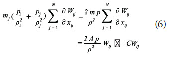
Equation 6 shows that the acceleration boundary deficiency is proportional to the total area of the deficiency as well as fluid pressure. Because cases of interest typically involve non-constant pressures equation 6 is not strictly suitable for use as a boundary correction. However proportionality to the kernel function for boundary deficiency can stil be observed even in cases in which a pressure gradient is present. Fig. 5 illustrates one such case. Shown in Fig. 5 is the vertical acceleration of a unity density fluid influenced by a downward body acceleration of unity magnitude.

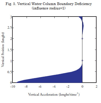
The pressure at the top of the water column is zero (gauge pressure), with pressure in the fluid varying as dp/dz=−ρg. The boundary deficiency in acceleration at the bottom of the water column still strongly correlates to the kernel function even in the presence of a pressure gradient. It is interesting to note that a boundary deficiency exists not only at the bottom boundary but also at the free surface. However, the low magnitude boundary deficiency at the free surface does not introduce substantial error as it typically results in only minor particle clumping.

Acceleration Boundary Deficiency Correction

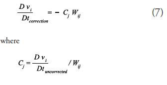
While an exact acceleration boundary deficiency correction could be gained by discerning the pressure gradient normal to a surface and analyzing the geometry of the deficiency, such an approach would increase computational complexity. Instead a simple -if inexact- correction is suggested in which the pressure is assumed to be nearly constant over the scale of the smoothing length. Then by assuming a known boundary acceleration, the relative fluidboundary acceleration in the absence of boundary forces can be calculated. If this relative acceleration is assumed to be the result of a boundary defi ciency then it can be corrected by applying a repulsive acceleration distributed as CWij away from the boundary. Where C is determined by choosing a sample particle, determining the relative particleboundary normal acceleration and dividing by Wij . To improve robustness it is advisable to average C over a small sample of nearboundary particles. Th is reduces correction error due to spurious pressure fl uctuations. Equation 7 shows this one dimensional acceleration boundary defi ciency correction with j representing a boundary particle index.

The assumption that a boundary acceleration is known is suitable for fi xed boundaries but requires an approximation when applied to freely moving boundaries. For objects with much greater density than the surrounding fluid, forward interpolation of acceleration is acceptable as object acceleration will change only slowly relative to the simulated timescales when acted on by fl uid forces alone. However, as relative object-fl uid density decreases, this approximation worsens. Further work is necessary to assess the impact of this assumption on low density object dynamic behavior.

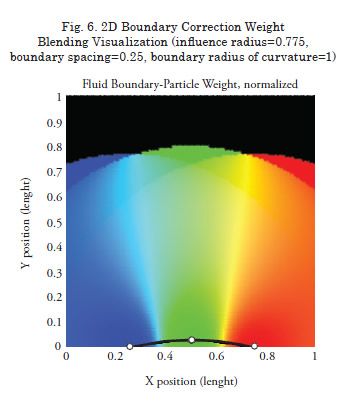
While the correction presented in equation 7 is suffi cient for one dimensional cases where a single boundary particle governs a boundary defi cient region, extension to higher dimensions requires a blending of corrections from multiple boundary particles. An empirical weighting function to blend correction values for two dimensional cases is shown in equation 8. Fig. 6 shows a visualization of the resultant weights.

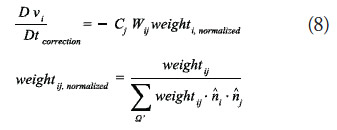
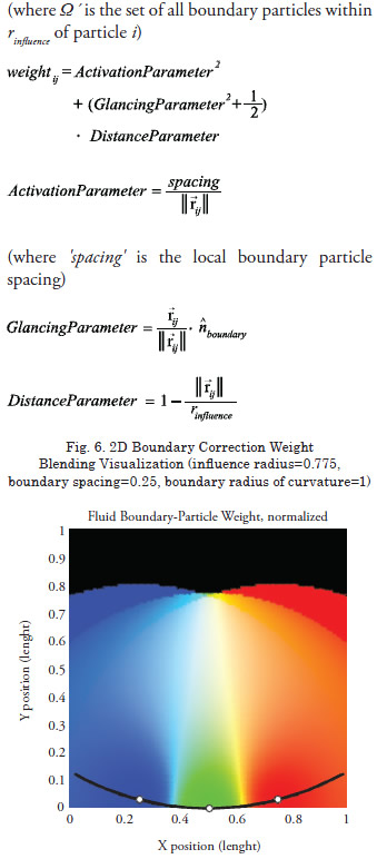
Fig. 6 illustrates the weighting scheme applied to simple concave and convex boundaries. Th e weights of the three boundary particles are shown by the blue, green, and red shades respectively.

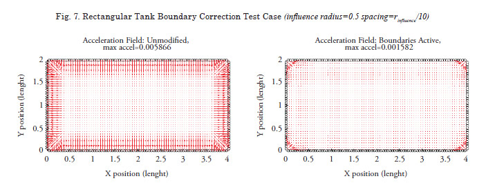
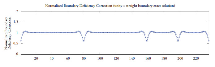
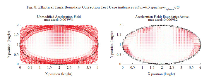
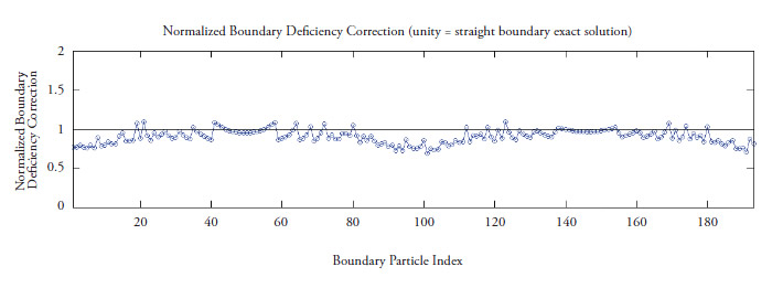
The boundary deficiency correction is applied to two test cases (one with a rectangular boundary, one with an elliptical boundary) each with constant pressure fluid. Fig. 7 shows the rectangular tank case.

Fluid pressure is unity with density=1000. Particle infl uence radius set to 0.5. Th e unmodifi ed acceleration fi eld is presented on the left and the corrected acceleration fi eld is shown on the right. Th e normalized acceleration correction magnitude for each boundary particle is shown in blue, and is plotted against boundary particle index (the zeroth boundary particle is located in the lower left with subsequent indexes moving counterclockwise about the rectangular tank). Fig. 8 shows the elliptical tank case with identical fl uid and simulation parameters.

Th e four dips in correction acceleration visible in fi gure 7 (rectangular case) are due to the change in boundary defi ciency due to the reduced volume of fl uid present near the four tank corners. Th e correction slightly overcorrects the boundary defi ciency in the sharp corners of the rectangular case. For the elliptical tank case, the acceleration present after boundary defi ciency correction near the high curvature sides of the elliptic tank represents an undercorrection of the boundary defi ciency and is likely a result of weighting function. Further refi nement of the weighting function may reduce the error in the correction due to geometry. Th e low curvature and straight sections show good correction of acceleration boundary defi ciency.

Because the correction presented emulates virtual particles, it alone is insufficient to act as a boundary condition. A secondary repulsion force such as the spatial repulsion force developed by Monaghan in 2009 [5] is necessary to prevent fl uid-boundary penetration. Th e presence of virtual particles or a boundary acceleration defi ciency corrective force can improve the behavior of spatial repulsive boundary forces. Th is is especially noticeable in the transient behavior present at the start of most simulations involving spatial repulsive forces alone. By correcting the boundary acceleration defi ciency immediately, near-boundary fl uid particles do not have to re-orient to allow for a spatial change to correct the boundary repulsion force.

Similar boundary acceleration correction work performed by Feldman and Bonet [11] does not require an assumption of a known boundary acceleration, but instead determines an acceleration correction by calculating the fl uid pressure gradient and assuming a known boundary geometry (straight or straight-corner). Further work is required to compare the relative performance of the two methods when applied to various cases.

Conclusions

Virtual particles are normally used to correct errors due to integral defi ciencies that appear in the governing equations near boundaries. Virtual particle behavior for deformable objects can be diffi cult to implement due to particle clumping after deformation. A simple repulsive correction which loosely emulates the presence of virtual particles in the momentum equation has been derived. An empirical weighting function to extend the theoretical boundary correction to higher dimension cases has been presented. Results obtained by applying the boundary correction to two constant pressure test cases were presented. Th e method yields good correction of acceleration boundary defi ciency in regions of low curvature but tends to slightly overcorrect at sharp corners and undercorrect near regions with high curvature.

Acknowledgments

The authors would like to express their gratitude to Dr. Pat Purtell and Ms. Kelly Cooper at the Office of Naval Research for their sponsorship of this work under grant numbers N00014-08-1-0695, N00014-10-1-0398, and N00014-07-1-0833.

References

[1] LUCY L. B. (1977), 'Numerical approach to testing in the fission hypothesis' in Astronomical Journal, 82 pp. 1013:1024.

[2] GINGOLD R. A. AND MONAGHAN J. J. (1977), 'Smoothed Particle Hydrodynmics: Theory and Application to Non-spherical stars' in Monthly Notices of the Royal Astronomical Society, 181:375-389.

[3] MONAGHAN J. J. (1994). 'Simulating free surface flow with SPH' in Journal of Computational Physics, 110:399-406.

[4] MONAGHAN, J. J.; KOS, A.; ISSA, N.. (2003) 'Fluid Motion Generated by Impact' in Journal of Waterway, Port, Coastal & Ocean Engineering, Nov. 2003, Vol. 129 Issue 6, pp. 250-259.

[5] MONAGHAN, J. J. AND KAJTAR, J.B. (2009) 'SPH particle boundary forces for arbitrary boundaries' in Computer Physics Communications, 2009, 180:1811–1820.

[6] LIBERSKY L. D., PETSCHECK A. ., CARNEY T. C, HIPP J. R. AND ALLAHDADI F. A. (1993), 'High strain Lagrangian hydrodynamics-a three-dimensional SPH code for dynamic material response' in Journal of Computational Physics, 109:67-75.

[7] RANDLES P.W., AND LIBERSKY L. D. (1996), 'Smoothed particle hydrodynamics some recent improvements and applications' in Computer Methods in Applied Mechanics and Engineering, 138:375-408.

[8] LIU, G. R. AND LIU, M. B.(2003). Smoothed Particle Hydrodynamics – a meshfree particle method, Toh Tuck Link, World Scientific Publishing.

[9] LIU G. R. AND GU Y. T. (2001), 'A local radial point interpolation method (LR-PIM) for free vibration analyses of 2-D solids'. Journal of Sound and Vibration, 246(1):29-46.

[10] LIU M. B., LIU G. R. AND LAM K. Y. (2002), 'Investigations into water mitigations using a meshless particle method' in Shock Waves 12(3):181-195.

[11] FELDMAN J. AND BONET J. (2007) 'Dynamic refinement and boundary contact forces in SPH with applications in fluid flow problems' in Int. J. Numer. Meth. Engng 2007; 72:295– 324.

[12] MONAGHAN, J. J. AND LATTANZIO J. C. (1985) 'A refined particle method for astrophysical problems' in Astronomy and Astrophysics, 149:135-143.

[13] P. G. TAIT, (1888) Physics and Chemistry of the Voyage of H.M.S. Challenger, Vol. 2, Part 4 HMSO, London.