Accreditation of Hydrodynamic Channels in use in Naval Modeling

Jorge Freiria^a

Abstract

This work considers a Quality System applied to a specific environment, the Hydrodynamic Towing Tanks or Channels, following the International Towing Tank Conference (ITTC) guidelines, gathered in turn from the international regulations, and it focuses the assessment of uncertainty in the experimental outcomes from the hydrodynamic tests called Test to resistance, as well as in determining which of the variables are those that have greater incidence on the mentioned outcomes.
En este trabajo se considera un Sistema de Calidad aplicado a un entorno específico, los Canales o Tanques de Ensayos Hidrodinámicos, siguiendo las directrices de la International Towing Tank Conference (ITTC), recogidas a su vez de la normativa internacional, y se centra en la evaluación de las incertidumbres en los resultados experimentales del ensayo hidrodinámico que se denomina Ensayo de Resistencia al Avance, y en la determinación de cuales variables son las que tienen mayor incidencia en dichos resultados.

Key words: Ship resistance, uncertainty evaluation, hydrodynamic tests

Resumen

En este trabajo se considera un Sistema de Calidad aplicado a un entorno específico, los Canales o Tanques de Ensayos Hidrodinámicos, siguiendo las directrices de la International Towing Tank Conference (ITTC), recogidas a su vez de la normativa internacional, y se centra en la evaluación de las incertidumbres en los resultados experimentales del ensayo hidrodinámico que se denomina Ensayo de Resistencia al Avance, y en la determinación de cuales variables son las que tienen mayor incidencia en dichos resultados.


Palabras claves: Buques, resistencia, incertidumbres, ensayos

________________________

^aFacultad de Ingeniería Instituto de Mecánica de los Fluidos e Ingeniería Ambiental
e-mail: jfreiria@fing.edu.uy

............................................................................................................................................................

Introduction

Research with physical models begins to be developed as a scientific instrument starting from the dimensional analysis theoretical development. Lord Rayleigh’s studies are the Pi theorem conceptual basis, which credit is done to E. Buckingham in 1914, (White, 1999). This way, the solution to hydraulic problems begins to be approached through its physical modeling to reduced scale. One of these problems, perhaps one of the most important problems of those times, given the fact that the economies of the nations depended upon the exchange of commodities by means of maritime transportation, was the decrease of resistance on the ships hulls.

William Froude was a pioneer in the fluid mechanics, applied to the determination and the reduction of this resistance. Froude realized the practical need of separating the resistance in components from different nature, developing the procedure which makes compatible the physical modeling with the dynamic similarity. In 1868 he published his paper “Comparison Law” establishing that the ratio between the ship’s residual resistance (due mainly to the waves formation) of similar dimensions were equal to the cube of the ratio of the linear dimensions, if their velocities were in an inverse ratio of the square root of their magnitudes. The need of knowing the frictional resistance or of viscous origin made him carry out research using flat plates completely submerged, finding an empirical formulation which permitted the development of the modeling and extrapolation of results to the prototype methodology (Todd 1967), with the construction of a test channel considered as being today’s existing installations forerunner.

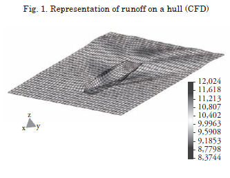
The introduction of computing tools in the fluid mechanics field has generated a substantial change in the simulation of runoff phenomena in general, and in particular in the fluids associated to the movement of a ship (Pérez Rojas, 1994). There are still some difficulties for its application due to a limitation imposed by the capacity of the machines used for its processing and post processing or the incorporation of more accurate models for the turbulence phenomena. The outcomes brought up through the numerical modeling with computers by means of the new CFD (Computational Fluid Dynamics) techniques, require in their development stage, a mechanism which permits the assessment of their degree of accuracy, generating new working lines which improve the output of the codes arriving even to propose different ways from those previously followed. The ideal tool for this action is to compare with the data obtained from the prototype itself. Nevertheless, this alternative is difficult to be implemented in the naval hydrodynamic field, which makes necessary to look into other information sources, in particular to outcomes brought up from the physical modeling carried out in test channels, being understood that these have proven their efficacy throughout the years, just as it has been previously mentioned.

As the capacity of the computers improves, the codes improve too, diminishing the modeling time and increasing their range, such as solving numerically Navier – Stokes’ equations with turbulence models. This, together with the improvement in the mesh systems, has permitted, evidently, to diminish those errors in connection with the results available in the hydrodynamic channels; this substantial improvement in the quality of the CFD outcomes generates an increasing exigency about the Test Channels outcomes, which is the source where the information for assessment of numerical models are provided from, demanding greater definitions and the assessment of errors or uncertainty in connection with the experiments. The assessment of these uncertainty, as well as the need of establishing a Quality Management System, demand the incorporation of the Test Channels to a universal Accreditation System.

Acreditation

Accreditation is the procedure through which an authorized Institution recognizes in a formal manner that an organization is competent to carry out a specific assessment activity. These institutions are in charge of assessing and carrying out an objective statement that the services and products meet some specific requirements. The Testing and Gauging Laboratories, the certification institutions (of products, of management systems, of people), the inspection institutions, and the environmental inspectors are examples of Competence Assessment Institutions.

Under the Quality outlines, for example, ISO 9000, the Certification or Registration terms, that point fundamentally to transparency in their procedures, for both the internal operation as well as for external relation. Otherwise, Accreditation requires, in addition, a level of competence in the performance of activities, which differentiates it from Certification or Registration. An example is the norm ISO/IEC 17025, “Requirements for competence of test and measurement laboratories”, which presents requirements of a higher degree of technical competence which include de determination of uncertainties.

Accreditation brings benefits to Management, since it offers an organization which is specialized and independent from the market interests that acts based on exclusively technical criteria. It puts to its disposal a valuable resource, a set of assessors who have proven their technical competence. It also strengthens the public’s confidence on the basic services (public health laboratories, safety of food, etc.). For the assessors, the benefit of Accreditation is the contribution that the logo “Accredited” offers as a distinguishing feature in the market, being an integrity and competence guarantee, hence increasing the trade opportunities. Nowadays it is an indispensible requirement in most activities, becoming a basic requirement in order to offer technical assessment services, such as measuring, certification of quality systems, etc.

Acreditation of Test Channels

The Test Channels utilized for hydrodynamic tests must be considered as Laboratories, where tests with physical models are carried out. This immediately suggests the incorporation of them into a quality and specific competence system, just as it is stated, for example, by the norm ISO 17025. Signs of involvement with this aspect of the measurement process are beginning to be observed, pressed, on one hand by the pressure exerted when quality systems are being implemented, and on the other hand due to the need of adjusting the uncertainty margins on the measures in order to validate the modeling outcomes carried out in CFD.

Leadership of this process has been for the International Towing Tank Conference (ITTC) that at the 22nd Conference indicates, in a formal manner, the need of the implementation of a quality and uncertainty in measurement estimation system. By means of their Quality Committee they establish an approximation to the issue through a clarifying document about the range and terms in connection with the assessment of uncertainty in measurement.

Historically the ITTC has proposed to go through the path of an improvement of the outcomes in order to ensure the required validation conditions, path which later on led to the certification of quality implementing a universal analogue system to that one developed in other areas, applied specifically to the Test Channels, their management and quality of outcomes.

The ITTC efforts towards improving the quality and validation of the information go back to 1960, when at the 9th Conference research with models normalized by some channels (ITTC, 1960, 2005) was promoted, and the submission of outcomes to the Committee of Resistance in accordance with the established in the Report was recommended. These installations agreed the test with these normalized models in order to determine variations in the measured resistance, and despite of the fact that some error sources were detected, errors were not determined, the dimensions of the models were not controlled and finally the effort was unsuccessful.

This issue is retaken at the 16th Conference, where four hulls were defined to carry out a joint research. These hulls were the Wigley, which is a hull with parabolic lines or mathematical careening, hull of series 60 with a 0.6 block coefficient, a Hamburg Ship Model Basin (HSVA) Tanker, and the Athena, a fast ship, a Cooperative Experimental Program (CEP) was established which would be working until arriving to the 18th Conference in 1987.

October 21, 1985 remains registered as the date of the creation of the Working Validation Party whose main task is to establish recommendations about that subject to the Committee, briefly outlining the foundations of the uncertainty calculation (ITTC, 1987).

At the 19th Conference, in 1990 the Validation Panel submits the “Guidelines for the Uncertainty Analysis in Measures” (ITTC, 1990) based on the norm ISO / ANSI together with examples related to tests in towing tanks.

The recommendations arisen from the Validation Panel are taken by the 20th Conference. Fundamentally, the responsibility for the activities related to the validation of data and the uncertainty calculation is transferred to the working parties, creating a Group whose action was focused mainly towards the establishment of a quality system in accordance with the norm ISO 9000. This Group was denominated Quality Control Group (ITTC, 1993).

The QCG’s task at the 21st Conference is focused on progressing on the concepts handled in a quality system, including examples of implementation (ITTC, 1996).
At the 22nd Conference, the problem of calculating the uncertainty and the validation is presented with more emphasis; in the Final Report and Recommendations, the Committee of Resistance states the following in its Chapter 5- "Analysis of Uncertainties in Experimental Fluid Mechanics" - (ITTC, 1999):

“The report of uncertainty in experiments continues to be a problem for the ITTC..... Those problems include the implementation of procedures, documentation and the submission of results. The estimation of the uncertainty associated with the experiments is indispensible for estimating the risks in design, not only when such information is utilized directly, but also, when it is used in the calibration and/or validation of other methods.”

Similarly, the Group submits a quality manual (ITTC, 2001) based on the norm ISO 9000, proposal which is submitted to the consideration as recommended procedure; in this manual procedures for calculating uncertainty in accordance with the normative developed by the American Institute of Aeronautics and Astronautics (AIAA) in 1995 are introduced based on the methodology described in Coleman & Steele (1989), being it an up-dating of the previous normative ANSI / ASME (1985), and of the international normative ISO GUM (Guide to the expression of Uncertainty in Measurement)

The Committee of Resistance adopts the recommended procedures about methodologies for the assessment of uncertainty, guidelines for the conduction of experiments in towing tanks and examples for the resistance tests presented in the Quality Manual: 4.9 – 03 – 01 – 01 “Uncertainty Analysis in EFD, Uncertainty Assessment Methodology”; 4.9 – 03 – 01 – 02 “Uncertainty Analysis in EFD, Guidelines for Resistance Towing Tank Tests”; 4.9 – 03 – 02 – 01 “Resistance Tests”; 4.9 – 03 – 02 – 02 “Uncertainty Analysis, Example for Resistance Test”

The 23rd Conference tells about the experience carried out by three laboratories, which taking into account the recommendations proposed at the previous call, carried out resistance tests, sinking and trim, and wave elevation, using models of the same geometry and test conditions, but of different scales; starting from these experiences, comparative data emerge for the variables utilized in the reduction equation and for determining reduction and for determining uncertainty. This work did not have enough details, did not take into account some effects affecting the total uncertainty, which meant the need of making new efforts in order to improve the individual uncertainty estimates (ITTC, 2002). Then, it is suggested a common methodology expressed through a series of procedures for the uncertainty analysis in the resistance tests, sinking and trim, wave profile and height, both for the simple tests as well as for the multiple ones. These procedures were included in the Quality Manual: 4.9 – 03 – 02 – 03 “Uncertainty Analysis Spreadsheet for Resistance Measurements”; 4.9 – 03 – 02 – 04 “Uncertainty Analysis Spreadsheet for Speed Measurements”; 4.9 – 03 – 02 – 05 “Uncertainty Analysis Spreadsheet for Sinkage and Trim Measurements”; 4.9 – 03 – 02 – 06 “Uncertainty Analysis Spreadsheet for Wave Profile Measurements”. This Conference recommends the carrying out of comparative tests between ITTC members, in order to identify systematic errors, action which was concreted at the 24th Conference, in which opportunity the laboratory members are invited to participate with such a purpose. An inter-comparison exercise was designed where two scales would be available (Geosims) of the model developed at the David Taylor Model Basin (DTMB) DTMB 5415, with length overalls of 5.720 m and 3.048 m respectively, which will be utilized by two groups of institutions for their tests and analysis. The DTMB 5415 is a model which represents a modern ship of “Combatant” type, widely used for CFD codes validation and uncertainty determination in EFD (Experimental Fluid Dynamics) selected in Gothenburg 2000 as a benchmark for validation of numerical models (ITTC, 2002, 2005).
Each one of the models will complete a pre–determined schedule which will take them to different laboratories, beginning at those laboratories where they were constructed, being these the Hydrodynamic Experiences Channel of El Pardo (CEHIPAR) in the case of model with a length of 5.720 m, and the CEHINAV of the ETSIN, for the model with length of 3.048 m (ITTC, 2005).

Uncertainty Determination - ITTC

The procedure adopted by the ITTC is based on the methodology defined by the AIAA in the Norm AIAA S – 071A - 1999 (1999) and by ANSI / ASME (1998), both founded on “Experimentation and Uncertainty Analysis for Engineers”, by Coleman, H.W. and Steele, W.G., as all of the methodologies and procedures source of reference and discussion.

It is necessary to introduce the concepts where the calculation of uncertainty on measurements is supported. Terms such as measure, error, uncertainty, can lead to misinterpretations or confusing interpretations if not clearly defined.

The definitions of the terms related to measurements are developed in the norm ISO/IEC/OIML/BIPM (1984) “International vocabulary of basic and general terms in metrology” (VIM), while the statistical concepts come from norm ISO 3534 “Statistics – Vocabulary and symbols” (ISO 1992,1999, 2006; AIAA, 1999; Schmid, 2000).

Measure: it is the subject attribute to measurement of a specific physical phenomenon which can be identified and valued. The clear identification of the measure and its detailed description from the point of view of the variables which take part in its definition is one of the main points in question. An incorrect or deficient definition could lead to failure in the measurement procedure.

Error: it is the discrepancy between a measurement and the true value of the measure. Two components are assigned to this magnitude, one component of random nature which is called “precision error” supposing that there are unpredictable variations affecting the measurement, and other one which reflects other aspects of the measurement which produce a slant and which is normally associated to non random effects, which is indicated as “systematic error”.

Uncertainty: doubt, fluctuation, irresolution, insecurity; in the case of the measurements it is applied with the sense of doubt or lack of certainty in the accuracy of the measurement outcomes. It is a parameter which characterizes the dispersion of values which can be attributed to the measure, reflecting the lack of an exact knowledge on the value of the measure. The contributions to uncertainty are attributed to several sources, being inevitable its existence; improvement of the measurement procedures can lead to diminishing the magnitude of the uncertainty, although they never disappear completely.

It is necessary to have a perfect knowledge of the principle of the measurement, this is, of the scientific foundation used in measurement, of the method or manner in which it must be carried out, and of the specific procedure for applying the proposed method. An inadequate knowledge of any of these aspects can lead to erroneous estimates both of the quantity measured and of its uncertainty. Among the possible uncertainty causes, supposing that both the measure and the method of measurement have been well defined and that the latter has been adequately executed, the following can be mentioned: incomplete knowledge of the environmental effects on the measure, personal predisposition of the observer in connection with a manipulation or reading of instruments, assigned values to constants, parameters used by the algorithms of the reduction equations, reference materials, etc., assumed hypothesis in the model and incorporated into the measurement system, repetition of experiments in conditions apparently identical.

Spreading of errors: Usually the desired magnitude is not measured directly but rather other variables which relate to one another, by means of the reduction equation, end up defining the desired value. The way in which such uncertainty affects the final measurement is called spreading of errors, and each one of its components must be assessed.

Type of Errors

The error is assumed to be integrated by two components, the first one associated to deviations in the procedures of measurement or “systematic errors”, while the remaining one attributed to countless aspects which in a random manner act during the procedure, is called “precision errors”.

Systematic Error: it is the total error component due to deviations or slants in the measurement procedure, for instance a slipping of the scale, influence of one of the magnitudes on the others, etc. There are three categories of systematic errors: associated to the calibration of the instrument or measurement system, to the gathering of data, and to the reduction of data. Within each category there can be several elemental sources which force the systematic deviation. The total value of the systematic error estimate is calculated using the root sum square (RSS). For example, for the variable there are J elemental sources of systematic errors identified by their estimators as , with which the systematic error in the variable can be calculated as:

Where is the estimate of the systematic error associated with the variable and are the estimates of the systematic errors which contribute the total systematic error; values must be estimated for each variable Xi utilizing the available information of the moment.

Spreading of Systematic Errors: the general expression of the uncertainty estimate due to the spreading of systematic errors of variables in the experimental measurement of magnitude r defined as is given by the expression:

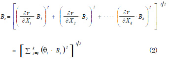
where is the systematic error corresponding to an experimental magnitude r and is denominated coefficient of sensibility, describes how sensible the measure is with respect to the variations of the corresponding input magnitude. Constants or properties of materials: the systematic errors associated with constants will be considered void since such data does not generate uncertainty. In the case of properties of materials which appear in the phenomena of reduction equations, when they are given in the tables or curves in according to a variable of definition. It will be assumed as systematic error in this case the error itself in the generation of such data. In case of not having access to this information, some criterion must be assumed, for example, considering the last meaningful figure of the values in the table.

Equations of calibration: The equation of calibration is an equation which relates a measurement or output value to the measurement of a magnitude or input value:

This equation must be treated as a reduction equation, and due to this, its treatment will be similar to that one given in equation [2]:

Precision Errors: the precision errors have their origin in an endless number of circumstances which cause different answers before the same measurement; these causes are always present and cannot be avoided completely. They include the operator and his/her answer facing each measurement, the instruments, the variations inherent to the energy supply, the environmental conditions which can produce variations in the answers of the instruments, etc.

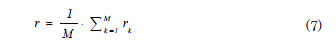
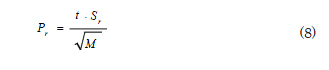
Estimate of precision errors: the precision error can be estimated in the measurement r as:

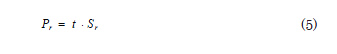
where t is the limit to the variable normalized for the established interval of confidence, known as range factor; for N>10 it is assumed a value t = 2 and is the standard deviation of the sample of N readings.

Spreading of precision errors: it has been previously established that the sources of precision errors are difficult to identify and are connected to different aspects of a very varied nature; however, it can be established that those errors have an absolutely random and Gaussian distribution.

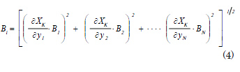
Assuming that M sources of precision errors have been identified for variable j; the general expression of the uncertainty estimate due to the spreading of precision errors is given by the following expression:

In the experiments whose results are obtained from a sole test, the precision limit of each variable must be determined. In order to do this, several ways must be taken into account: repeated measurements, auxiliary tests, previous experience, estimate starting from the data of the scale, etc.

When multiple samplings are carried out, averaged values of the M sets of measurements can be determined, in the same conditions of the experimentation, from which it is deducted

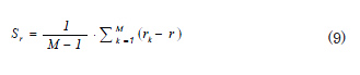
The limit of the precision error of the set of samples is transformed into

being the standard deviation of the sample

Test Channels: Uncertainty in measurements in the Resistance Test

The resistance test consists in conducting a model to a predetermined speed with the finality of determining the value of the resistance of the careening. To these effects, the resistance of the model as well as the velocity must be measured in a simultaneous way (ITTC, 2002). Once the total resistance has been determined the component denominated residual resistance must be deducted, which is that one which keeps the same in model and prototype if Froude’s conditions of modeling of equality of number are respected; with this value and the estimate of the viscous component the total resistance in the prototype is finally determined.

The resistance is the horizontal component of the opposite force that the fluid exerts on the hull, and it is determined through the measurement of the tension force. To measure this quantity different methods are used, for example, mechanical or electronic dynamometers, load cells, etc.

The advance velocity of the model cannot be measured or it is very difficult to measure directly, for this reason, it is decided to measure the velocity of the dynamometric car, which is generally obtained through an encoder. This could be directly coupled to one of the wheels of the car or to one device bound to the car which can rotate without slipping by one of the third rails.

The density and viscosity of water affect the outcomes of the test, so they must be defined each time. Their determination is done in an indirect manner, by means of the measuring of the water temperature corresponding to the moment the test is being executed.

The measurement of the coefficient of resistance is expressed in a dimentionaless way which is being given by the equation

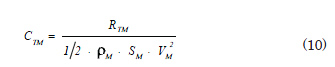
where is the measured resistance, is the density of water during the test, is the model wet surface and is the measured velocity, corrected by blockage if necessary.

The value of the determined residual component, dependent upon Froude’s number, whose calculation is carried out using the expression

where is the sample coefficient of resistance, is the frictional coefficient of resistance given by the model – ship Correlation Line adopted by the ITTC in 1957, k is the form factor deducted by the Prohaska method (ITTC 1966).

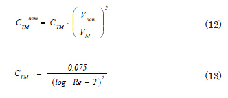
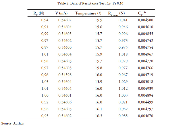
The tests are designed for a nominal velocity , but this velocity can hardly be obtained in an accurate form in the tests, hoping to find very close values in a normal distribution which will depend upon the quality of the equipment, of the calibration of the same, and the expertise of the operator. Given the fact that in this exercise the outcomes for the pre-established nominal velocity must be compared, the true velocity must be corrected, taking into account that for little variations of same, the fact that the resistance is proportional to the square of the rate between velocities (ITTC, 2000).

being Reynolds’ Number for the test conditions, where is the velocity of the model, is the length of the model and is the viscosity of water.

In addition, the ITTC establishes the need of using a normalized temperature for the submission of outcomes due to the great dependency of the resistance on the viscosity (ITTC, 2002, 2005). In the case of the tests carried out for third parties, it is recommended to normalize to the medium temperature of the set, while in comparison exercises such the one proposed, the temperature will be corrected to a normalized temperature of

where is the residual resistance and , are the corrected coefficients for the normalized temperature.

The frictional resistance is dependent on the temperature, but not so the component of resistance by wave formation, which is calculated using the data as they come from the corrected tests for the nominal velocity. Equation (14) can be expressed in the following manner taking into account (11)

where is the total normalized coefficient of resistance, is normalized coefficient of friction and k is the factor or form.

Experimental determination of coefficients in exercise proposed by the ITTC

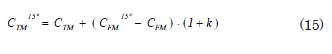
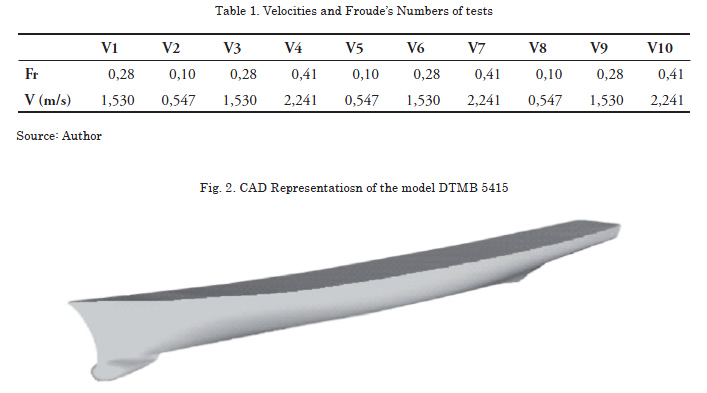
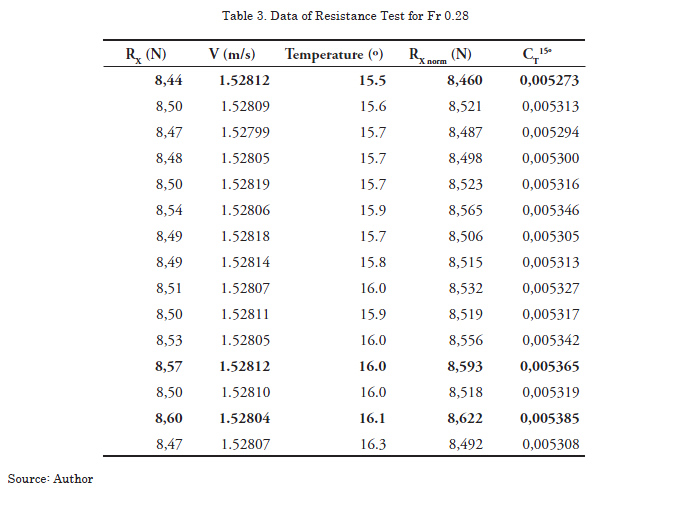
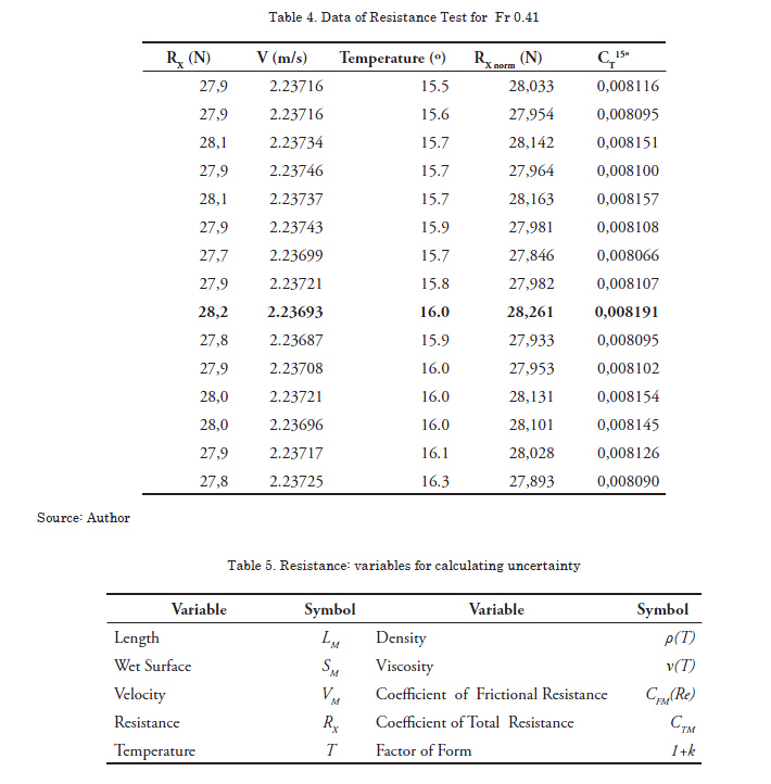
The outline of the tests, which were carried out in five consecutive days, is shown in detail in Table 1. The initial run will only be taken into account for generating an initial movement of the water in the tank. In Table 2 to Table 4 experimental outcomes obtained with model DTMB 5415, are shown. This model has been designated by the ITTC as a test model (benchmarking), at the Channel of Naval Hydrodynamic Experiences (Canal de Experiencias Hidrodinámicas Navales (CEHINAV) ) at the Naval Engineers Superior Technical School (Escuela Técnica Superior de Ingenieros Navales (ETSIN) in the Universidad Politécnica de Madrid (UPM), participant in the international comparison exercise. This model has the following principal dimensions at the floating: length 3.048 m, beam 0.410 m, draft 0.132 m.

The first three columns represent the gross data obtained from the tests, while in column 4 the values of resistance corrected for the nominal speed are shown, and finally in the last column, the values of the coefficient of resistance normalized for a temperature of 15º are transcribed. Once the set of coefficients has been determined, depuration through the application of statistical methods is carried out. (Eliminated data in bold).

Analysis of Systematic Errors

In order to determine uncertainty in the resistance outcomes, the limit of the systematic errors must be established for the following set of variables:

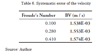
Length: It is assumed that in the confection of the model an error of ± 1 mm is made when the machine for carving the model on wood starts the process, for example, on the fore end, and another error exactly the same when it finishes on the opposite end, due to an error in the positioning of the cap. The systematic error would be = 2.000E-03 m.

Wet Surface: we will have contributions due to errors transmitted by the weighing of the model generating an error in estimating the displacement, and due to the errors made in the linear dimensions which act in the same direction, completing a systematic error = 4.154E-03 m2.

Velocity: the velocity is the measurement through an encoder coupled directly to the dynamometric car motive system. Since there were not up-dated data on how it functioned, data on calibration of the system were handled, finding out that the errors combined of calibration and of the reduction equation (V=d/t; d is the distance and t is the time in covering such distance) are:

Resistance: The resistance is measured through the load cell which is connected by means of a flexible link directly to the model. In this case there appear components of error associated with calibration of the cell itself and different sources in the acquisition of data (misaligning of the load cell, analogous - digital conversion of the measuring and trim equipment of the model). The composition of these errors determines a systematic error = 4.361E-02 N.

Temperature: it is measured with a microprocessor thermometer which consists of a calibrated termistor. The temperature termistor is linearized by means of a microprocessor fitted in the instrument. The range of the measurement is between –50º and 150º, being its resolution 0.1º and its precision ± 0.4º. This value is considered as an estimate of the error in this case, being then = 4.000E-01º.

Density: it is calculated according to the tables provided in the ITTC “7.5-02-01-03 procedures. Density and Viscosity of Water”, whose values can be represented by the correlation:

where t is the temperature of the water channel measured in ºC; part of the systematic error is associated with the equation of reduction of the phenomenon, while the adjustment curve of the experimental data contributes with another component. Finally the estimation of the error will be

Viscosity: analogously like in the case of density, viscosity is calculated according to the tables provided in the ITTC “7.5-02-01-03 proceedings. Density and Viscosity of Water”, whose values can be represented by the correlation:

where t is the temperature of the water of the channel measured in ºC. The components of error are conceptually equivalent, completing in this case a value of

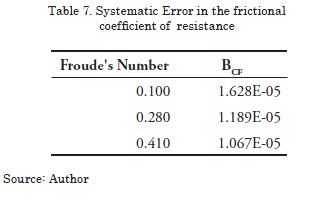
Frictional Coefficient: it is calculated through equation 13, being the error limited to that one associated with the equation of reduction:

being its values according to the velocity the following:

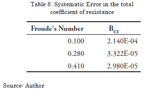
Total Coefficient of Resistance: it is calculated through equation 10, and its systematic error is also associated with this equation of reduction like in the previous case:

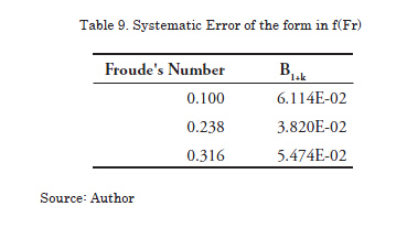
Form Factor: this factor was estimated in an experimental form according to the established in the ITTC, 1999; the reduction equation of these data leads to an estimate of its systematic error shown in the following table:

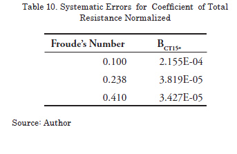
Coefficient of total resistance: it is calculated through equation 16, and like in the previous cases the estimate of the systematic error is associated with this reduction equation, being the values

Analysis of Precision Errors

In order to determine the resistance, the magnitudes which show the random variation are: velocity, resistance, and temperature.

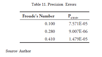
However, when correcting the experimental values to velocities and temperatures, the only variable affected by the precision errors will be the resistance. Given the fact that multiple tests have been carried out for each velocity, it is necessary to consider as a multivariable experiment, according to which we will have that the precision rate must be calculated in accordance with the formulation established in equations 8 and 9. The processed data for the three velocities are detailed in tables 2 to 4. The criterion adopted for dropping observations out of the range was to consider, in order to eliminate them, those measurements which exceeded ±2σ the average [34], eliminating three records Fr = 0.28 and one for Fr = 0.41 (shown in bold). [σ represents the standard deviation of the sample]

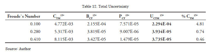
The uncertainty associated with the coefficient to total resistance normalized, UCTM15º, is calculated using the quadratic mean (root sum square) applied to the quantities which are involved in the phenomenon, the estimate of the systematic error , BCT15º, and the estimate of the precision error, PCT15º. In the last column of Table 12, how much the uncertainty calculated with respect to the total value of coefficient represents is shown with respect to the total value of coefficient CTM15º (second column).

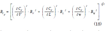
Spreading of Errors: Analysis of Sensibility

Complementary to the estimate of uncertainty, the need of having, on one hand, an automated procedure which permits the assessment of uncertainty in real time, and on the other hand, to

count on, with tools which permit the measuring of the influence the errors from the different variables have on the total value, was presented, generating useful information for the improvement of the processes or instruments (Longo y Stern, 2005).

The basic idea of this procedure can be explained through the description of the complex system of variables which is involved in the experimental tests and which is shown in Fig. 3. A first level is constituted by environmental variables completely independent; in this group we can distinguish environmental variables which define the environment of the experimented, other variables which define the dimensional frame, and finally those which are involved with the adjustment of the system of the collection of data and operation of the system.

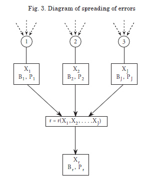
The set of variables of the first level act determining of conditioning those of the middle level which are those which have been identified as direct responsible for the variation of the magnitude which is intended to me measured. These latter determine the outcome of the experiment or test through a superior level or directly in its incidence in an equation of reduction, which is a mathematical model developed in order to quantify the phenomenon.

In this equation of reduction normally emerges from a process of an dimensionaless analysis evaluated at the light of experimental data. In these cases, the determination of uncertainty in the resulting measurement is a high complexity task, where the errors associated to the measuring of the variables of the initial level are transmitted to the recording variables, and the composition of uncertainty of these latter define through the equation of reduction the uncertainty of the final outcome.

Assessment of uncertainly in "linked steps"

The proposition of using the outline described calculating the systematic errors of the elemental variables or of initial level, using these outcomes to next calculate the corresponding errors in the recording variables, finishing the process through calculating the systematic error in the control magnitude using the previous values, all through an automated process so that a variation in any initial value is automatically reflected in the final outcome.

The proposed outline applied to the resistance test is described below, beginning from the superior level. The outcome of the resistance test is the resistance coefficient normalized . This coefficient is described in the equation of reduction according to other test variables, which represent the physical phenomenon, being this the superior level of the “linked steps” analysis. Each one of the factors involved in the previous equation represents the variables of the middle level: , k (defined experimentally), which depend upon the quantities measured or recorded: resistance, density, etc. Finally, these latter are determined by elemental variables which depend upon external factors: from the process of elaboration of the model (L), from the environmental conditions, (T), ν = (T), or from the operational aspects such as the system of gathering of information in the case of or the calibration of the measuring system of velocity V.

Analysis of Sensibility for tests at the CEHINAV

In order to demonstrate how the variation of the systematic error influences the outcome of a variable, a test velocity corresponding to Fr = 0.280 as reference, has been chosen, including each time the modifications compared to the values determined in the tests (Table 13).

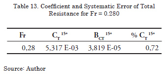
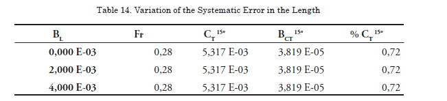
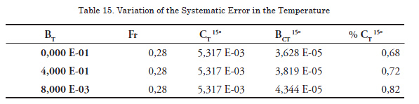
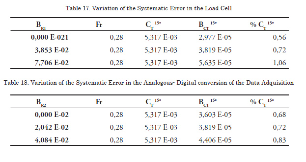
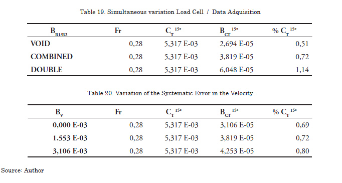
The values of the systematic errors of the selected variables are modified manually in the calculation program. Using the analysis procedure, those errors are forced in two opposite situations, duplicating them in first place and then reducing them to zero. The results of these modifications are shown below:

Analyzing the data presented for the variations of systematic errors and their incidence on the total uncertainty it can be established that the combination of two factors, the load cell and the data finder, supposes the most important factor to take into account in view of the limitation of the uncertainty. On their side, the variation of the error in the temperature, the weighing of the model, and the velocity have meaningless incidence, while the variation in the error made in determining the length is significant.

Conclusions

Assessment of uncertainty associated to the coefficient of resistance in the Test of Resistance for the experimental installation involved in the uncertainty determination exercise at an international level was presented. Basic aspects of the theories and procedures involved in such calculation were included.

This work is intended for the spreading of practices involved in the Accreditation of experimental laboratories as well as to promote the Test Channels which are not involved in instances such as the ITTC and to include them in their procedures.

On the other hand, the importance that the operator has in the identification of the systematic errors is presented, including the bases of an automated procedure which has been denominated “analysis in linked steps”, becoming a tool which not only permits the determination in real time of the uncertainty associated to each one of the tests in particular, but also as an objective means of identification of the elements of greater weakness of the procedure or of the installation in order to be able to act on them as well as to improve the measurement system.

References

[1] TURSINI, L. Transactions INA, vol 95, 1953.

[2] WHITE, F.M. Fluid Mechanics. McGraw – Hill, 1999.

[3] TODD, F. H. Resistance and propulsion. Principles of Naval Architecture, 1967.

[4] PÉREZ ROJAS, L. Los CFD como herramienta en Hidrodinámica. Aulas del mar. Universidad de Murcia, Cartagena, Septiembre 1994

[5] CURA, A., BERTRAM, V. Métodos de CFD en modelación naval. Facultad de Ingeniería, Montevideo, Uruguay. 1995.

[6] ITTC. 9th International Towing Tank Conference. Proceedings; Decisions and Considerations 725. Paris, Francia. 1960.

[7] ITTC. 17th International Towing Tank Conference. Proceedings 79 - 88. Gotenburgo, Suecia. 1984.

[8] ITTC. 18th International Towing Tank Conference. Proceedings 311 - 316. Kobe, Japón. 1987.

[9] ITTC. 19th International Towing Tank Conference. Proceedings V1. 578 - 603. Madrid, España. 1990.

[10] ITTC. 20th International Towing Tank Conference. Proceedings V1. 79 - 103. San Francisco, USA. 1993.

[11] ITTC. 21th International Towing Tank Conference. Proceedings V1. 315 - 337. Trondheim, Noruega. 1996.

[12] ITTC. 22th International Towing Tank Conference. Resistance Committee: Final Report and Recommendations to the 22nd ITTC. Seul, Japón. 1999.

[13] ITTC. 22th International Towing Tank Conference. Sample Quality Manual. Seul, Japón. 1999.

[14] ITTC 22nd. International Towing Tank Conference, Resistance Committee Report, ITTC, 1999. Seoul, Corea.

[15] ITTC. QM Recommended Procedures. Performance, Propulsion; 1978 ITTC Performance Prediction Method. 1999.

[16] ITTC. 23th International Towing Tank Conference. Proceedings; Resistance Committee: Final Report and Recommendations” 17 - 87. Venecia, Italia. 2002.

[17] ITTC. QM Recommended Procedures. Testing and Extrapolation Methods; Resistance; Resistance Test. 2002.

[18] ITTC. QM Recommended Procedures. “Resistance Uncertainty Analysis, Example for Resistance Test”. 2002.

[19] ITTC. 24th International Towing Tank Conference. Proceedings V1. 313 - 321. Edimburgo, Inglaterra. 2005.

[20]ITTC. 24th International Towing Tank Conference. ITTC Worldwide Series for Identifying Facility Biases. Edimburgo, Inglaterra. 2005.

[21] INTERNATIONAL ORGANIZATION FOR STANDARDIZATION. ISO/IEC PRF Guide 99 International vocabulary of basic and general terms in metrology (VIM). 1999.

[22]INTERNATIONAL ORGANIZATION FOR STANDARDIZATION. ISO 3534 – 1 Statistics – Vocabulary and symbols. 2006.

[23]INTERNATIONAL ORGANIZATION FOR STANDARDIZATION. ISO/TAG 4/WG3: 1992. Guide to the Expression of Uncertainty in Measurement. 1992

[24]AMERICAN INSTITUTE OF AERONAUTICS AND ASTRONAUTICS. AIAA S-071 Standard. Assessment of Wind Tunnel Data Uncertainty. 1999.

[25] SCHMID, W. A.; LAZOS, R. J. Guía para estimar la incertidumbre de la medición. CENAM, El Marquez, Qro., México. 2000.

[26]COLEMAN, H. W.; STEELE, W. G. Experimentation and Uncertainty Analysis for Engineers; John Wiley & Sons, Inc., New York, NY. 1999.

[27]LONGO, J.; STERN, F. Uncertainty Assessment for Towing Tank Tests with example for Surface Combatant DTMB model 5415. Journal of Ship Research, Vol. 49, No. 1. Marzo 2005.

[28] CEDEX (Centro de Estudios y Experimentación de Obras Públicas) - Ministerio de Fomento (http://www.cedex.es/).

[29]ENAC. Acreditación, una herramienta al servicio de la Administración y de la sociedad; información institucional. Entidad Nacional de Acreditación (http://www.enac.es/)

[30]ENAC; La Entidad Nacional de Acreditación; información institucional. Entidad Nacional de Acreditación (http://www.enac.es/)

[31]ENAC. Laboratorios Acreditados: la necesidad de estar seguro; información institucional. Entidad Nacional de Acreditación (http://www. enac.es/)

[32] PEREZ ROJAS, L; VALLE CABEZAS, J.; SOUTO IGLESIAS, A. The future in the experimental ship hydrodynamics. ETSIN. 2nd International Conference on Maritime Transport and Maritime History: Maritime Transport 2003, Barcelona, España. Noviembre 2003.

[33]LÓPEZ GONZÁLEZ, L. A.; PEREZ ROJAS, L. Estimación de la incertidumbre en la medida del hundimiento y trimado del modelo Serie 60. Universidad Politécnica de Madrid, ETSIN. Madrid, España. Octubre 2002.

[34]CERNUSCHI, F.; GRECO, F. I. Teoría de errores de mediciones. Editorial Universitaria de Buenos Aires. Buenos Aires, Argentina. Junio 1974.

[35] Proyecto Bajel: Informe de los ensayos de resistencia realizados con el modelo de la carena del buque “Serie 60”. Estudios de Incertidumbre. Departamento de Arquitectura y Construcciones Navales, Canal de Ensayos Hidrodinámicos, ETSIN. Noviembre 2000.

[36]BADANO, P.; GUARGA, R. Las técnicas de modelación en canales de prueba navales: estudio de la viabilidad de su aplicación en el Canal Hidrométrico del IMFIA. Facultad de Ingeniería, Montevideo, Uruguay. 1990

[37]PROHASKA, C. W. A simple method for the evaluation of the Form Factor and Low Speed Wave Resistance. Proceedings 11th ITTC, 1966.