Ship Science & Technology - Vol. 15 - n.° 30 - (47-57) January 2022 - Cartagena (Colombia)
DOI: https://doi.org/10.25043/19098642.228
Nicolás Ruiz 1
Bharat Verma 2
Luís Leal 3
Mauricio García 4
1 COTECMAR. Vía Mamonal Km. 9. Cartagena, Colombia. Email: nruiz@cotecmar.com
2 COTECMAR. Vía Mamonal Km. 9. Cartagena, Colombia. Email: bharat@cotecmar.com
3 COTECMAR. Vía Mamonal Km. 9. Cartagena, Colombia. Email: lleal@cotecmar.com
4 COTECMAR. Vía Mamonal Km. 9. Cartagena, Colombia. Email: mgarcian@cotecmar.com
Date Received: August 30th, 2021 - Fecha de recepción: 30 de agosto del 2021
Date Accepted: November 27th, 2021 - Fecha de aceptación: 27 de noviembre del 2021
For the design of naval ships, the operational environmental conditions in which ship navigation will take place must be taken into account. The present study presents the effect of shallow water on ship'sdrag. Numerical simulations using Computational Fluid Dynamics with the Star CCM+ Commercial Software has been performed for sea depths in which the BCFBC Shallow Draft River Combat Boat will perform operations. A full-scale validation campaign of the simulations with the built boat has been developed. The shallow water effect on ship total resistance and the residual resistance for different depths and speed has been evaluated.
Key words: Computational Fluid Dynamics CFD, Ship Resistance, Shallow Waters, Experimental Fluid Dynamics.
En el proceso de diseño de las embarcaciones militares se deben tener en cuenta las condiciones del ambiente operacional en el cual se desarrollarán las operaciones. En este artículo científico se estudióla afectación de la resistencia al avance debido a las aguas poco profundas. Realizando simulacionesnuméricas mediante Dinámica Computacional de Fluidos con el Software Comercial Star CCM+ en las profundidades en las cuales realizará las operaciones un Bote de Combate Fluvial de Bajo CaladoBCFBC. Se desarrolló una campaña de validación a escala real de las simulaciones con el bote construido.La afectación de la resistencia al avance total y la resis- tencia residual para distintas profundidades yvelocidades fue analizada.
Palabras claves: Dinámica Computacional de Fluidos CFD, Resistencia al Avance, Aguas poco profundas, Dinámica de Fluidos Experimental.
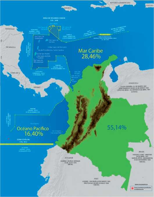
The Science and Technology Corporation for the Naval, Maritime and River Industry COTECMAR has been characterized by promoting, leading and promoting the interest sand maritime power of the country. Colombia is a country with a large maritime and fluvial extension, with more than 928,000 km2 of maritime area and a fluvial extension of 24,725 km of rivers, 75% of which are navigable. The Colombian Navy is in charge of the surveillance and control of this large fluvial extension, which through the Marine Infantry is present in these areas. Colombian rivers are characterized by different soil conditions, water characteristic sand depths that change in winter and summer. Considering the above, there is a need for river resources that allow for continuous navigation and military operations, even when river levels are very low in the summer.
To meet this operational need of the Colombian Navy, COTECMAR designed and built a Low Draft Fluvial Combat Boat (BCFBC), which meets the operational needs required by the Marine Infantry, thus allowing navigation and the development of military operations in shallow secondary and tertiary rivers during the winter and summer, generating a new capability for the Colombian Navy.
The design of such a boat entails the challenge of analyzing and determining the shallow-water drag effect for planing hulls. Hydrodynamic phenomenon that has been the subject of some numerical and experimental studies [1]. These studies are of great importance to determine the installed capacity required to meet the design requirements associated with this high operational demand.
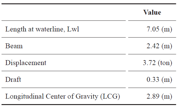
In this study, full-scale numerical simulations of the BCFBC were made at different depths by Computational Fluid Dynamics CFD, using the commercial software Star CCM+, which is a multiphysics simulation tool for simulation of designs in real conditions, using finite volumes. In addition, a validation campaign was developed with experimental tests on the vessel once built at different depths to verify its performance. The characteristics of the boat are listed in Table I.
Table 1. Parameters of FAC.
Complex flows governed by turbulent effects with high Reynolds numbers and unsteady flows with large fluctuations in space and time such as those of Naval Hydrodynamics are governed by the Navier Stokes equations. Different methods have been proposed to capture these phenomena, which are characterized by the formation of turbulence at different scales, which generate a transfer of energy from large to small. These phenomena can be calculated by Direct Numerical Simulation (DNS), Large Eddy Simulation (LES) and using the Reynolds-Averaged Navier Stokes Equations (RANS) in which turbulence is modeled at all scales. Currently, in Naval Hydrodynamics the most commonly used method is RANS, providing a sufficiently accurate solution and with a reasonable computational and meshing capacity compared to DNS and LES.
Starting from the mass continuity equation and under the assumption that only incompressible flow is considered, Equation 1 can be written removing the influence of density as Equation 2.
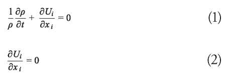
Therefore, the Navier Stokes equations can be written as follows:
Where σij is the total tension of a Newtonian Fluid.
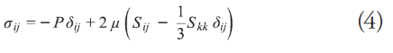
where the strain rate Sij is defined as follows
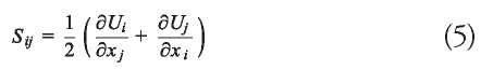
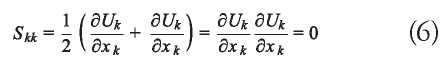
for an incompressible flow, Skk in Equation 4 is zero.
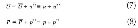
using the Reynold's decomposition, dividing the instantaneous speed Ui and the pressure P into an average and fluctuating component U, P, u”, p"
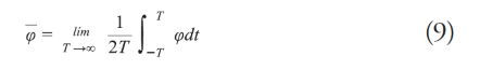
The time average of a variable is defined as
Using averaging properties, we obtain the continuity equation

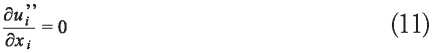
Subtracting Equation 10 from Equation 2, we obtain that the fluctuating speed also follows the continuity equation
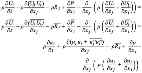
From the Navier Stokes equations over time we obtain:
Assuming that the fluid is incompressible, the continuity equation is expressed as follows
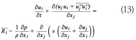
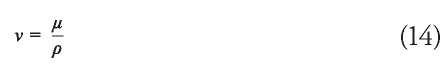
where v is the kinematic viscosity
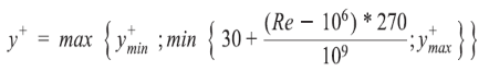
The turbulence model used in the simulations was the two-equation k-ω SST which uses the k-ω model in the boundary layer being the region that is dominated by viscosity and the k- E model outside this region. Thus, it provides more realistic flow solutions in the boundary layer which is achieved with a change function. For all simulations in this paper a high Reynolds number model or Wall Function was used, the value of y+ is dependent on the Reynolds number and consequently for high Reynolds numbers the higher this value should be. The calculation of this value was performed following the recommendations of Numeca [6] taking as reference the highest speed of the analysis.
The computational domain was defined following the ITTC recommendations [2] for planing vessels Fig.2, placing the boundaries far enough apart to avoid affecting the solution, the computational domain defined is four lengths aft, three lengths forward and three lengths to the side. In order to reduce the computational domain and computational time, the simulations were performed at half-length by applying the symmetry condition. Commonly,in drag simulations certain degrees of freedom are allowed to the rigid body, for the case of study pitching and heaving movements were allowed.These movements are significant in planing boat sand therefore require meshing techniques that allow for high body movements without affecting the solution. The movement in the X axis of the rigid body was not allowed and the speed was imposed on the flow in the opposite direction to the motion in order to obtain the forces to which the body is subjected, thus obtaining the drag.
Fig. 2. Domain and Boundary Conditions.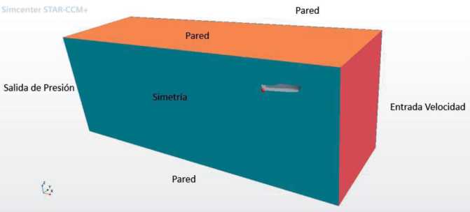
In these simulations, the computational domain was divided into two regions using Overset Mesh, which is used for bodies that undergo high motions. A base or subsequent stationary domain was generated, as well as a domain called Overset, which follows the rotation and other movements of the boat, generating an interpolation between the cells of these two domains during the simulation to obtain the solution.
Shallow Water SimulationsIn shallow water simulations it is necessary to consider some physical effects that are negligible indeep water theory, particularly the viscous effects on the bottom and the rigid body, so the bottom boundary condition must be imposed as no-slip, causing a gradient in the flow speed to be generated. For such purpose, additional meshing layers are added on this boundary, thus increasing the total number of cells in the computational domain.
Fig. 3. Deep Water Meshing.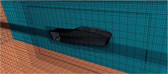
The definition of the meshing in Shallow Water is different from traditional drag simulations, considering the proximity of the boat to the bottom (computational volume limit), for this case the Overset Mesh cannot be used since due to the displacements of the rigid body, the moving region could be outside the base domain, preventing to obtain a solution. For this reason we used Morphing Mesh with a single region which allows the deformation of the mesh depending on the movements to which the rigid body is subjected.
Fig. 4. Shallow Water Meshing.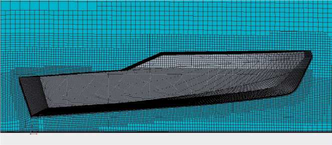
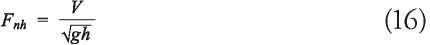
The drag in shallow water differs significantly from the drag in deep water and is therefore a determining factor in the design of this type of vessel. These drag effects are evidenced by the vessels based on their length-to-depth ratio L/h, therefore these boats experience them permanently during the normal course of their operations. Experimental, theoretical and numerical simulation references indicate that these effects begin to appear at depth Froude numbers Equation 16 greater than 0.7, with a peak of maximum effect at a depth Froude number of 0.95 and persist up to Froude numbers of 1.2, identifying three regions of effect as shown in Fig. 16. 5 [3]:
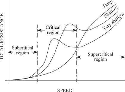
The navigation area of these boats is characterized by the variation of their depth, with depths varying between 0.5 and 5 meters. Fig. 6 shows the subcritical, critical and supercritical regions based on speed and depth, evidencing that this vessel has a permanent drag effect when navigating in these regions and therefore it is a critical factor to comply with the contractual speed in all its operation areas.
Fig. 6. Velocity-Depth curve with critical regions.
Numerical simulations to assess drag were carried out at the depths shown in Table 2, where they are expressed in the length-to-depth ratio L/h.
Table 2. Simulation depths..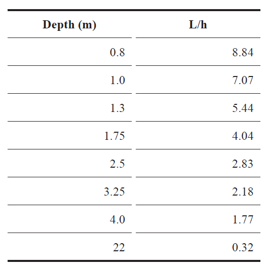
Simulations were performed on Star CCM+ using a 128-core @2.25GHz server. These were carried out for the depths mentioned above and speeds upto 21 knots. The results of the drag are shown in Fig. 7, which shows a considerable drag effect based on the depth, increasing significantly and running the characteristic peaks of the drag curve of planing boats at lower speeds with decreasing depth.
Fig. 7. Total Drag-Speed curve at different depths.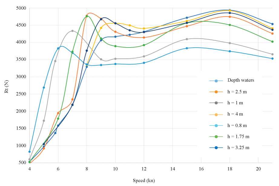
As mentioned above, one of the biggest challenges identified during the design of this vessel was to reach the maximum design speed of 15 knots, it is evident that the drag in deep water for this speed is similar to the drag obtained for significantly lower speeds at shallower depths; between 7 and 9 knots,and therefore it is of vital importance since the installed capacity was limited to 120 Hp, resulting in the risk that it would not be enough to exceed these drag peaks at all depths.
In order to guarantee this design speed, a prototype boat was built and subjected to performance tests at different depths, and a hydrodynamic optimization of the shapes was carried out, reducing the drag by 8% for the design speed. The drag was assessed for a total of 300 variations of the prototype hull usinga semi-parametric variation of shapes, and the drag values correspond to the hull selected after applying an optimization process, which is not described in this paper. To further analyze the effect on shallow water drag, it is more convenient to plot drag based on Fnh to identify the subcritical, critical and supercritical regions. Fig. 8 shows that the greatest drag effect corresponds to the values mentioned in [3], reaching a greater effect at Fnh = 0.95. Itis also evident that after the supercritical regiona reduction in drag is obtained, which generates an increase in the final speed of the vessel when exceeding this region.
Fig. 8. Total Drag-Fnh curve.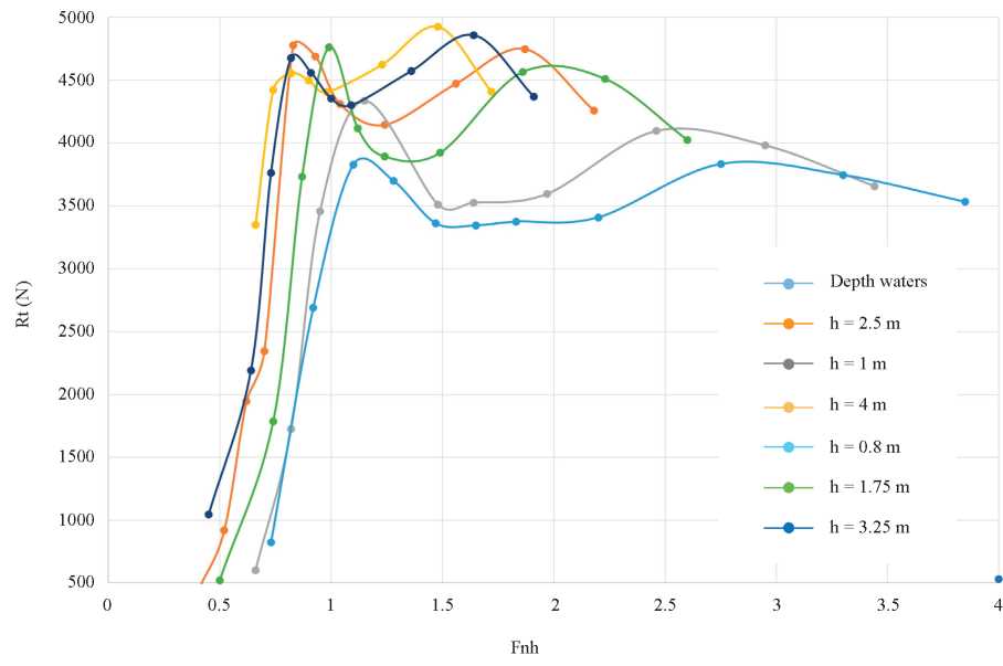
It is important to analyze the impact of the drag due to these phenomena, and it is convenient to separate the components of the total drag calculated by the numerical simulations to study them in detail. Separate monitors are used for viscous drag RV and residual drag RR. The increase in drag in shallow water is mainly due to residual drag, the effects on viscous drag can be neglected [3].
A convenient way to analyze the residual drag obtained in the simulations is to express it as theratio between the residual drag in shallow waterand deep water based on the Fnh number.
From Fig. 9 it can be observed, based on the ratio of shallow and deep water residual drag and the Fnh number, that the drag increase in the regions of distress due to shallow water effects is a function of the ratio of hull length to the depth L/h, as is the subsequent drag reduction when passing these regions as expressed by Millward in 1986, with a considerable increase in drag when this ratio has higher values in the critical regions [4]. In the experiments performed by Millward this ratio was limited to a value of L/h = 6, the simulations were carried out at a maximum value of L/h = 8.8 corresponding to a depth of 0.8 meters.
Fig. 9. Total Drag-Fnh curve.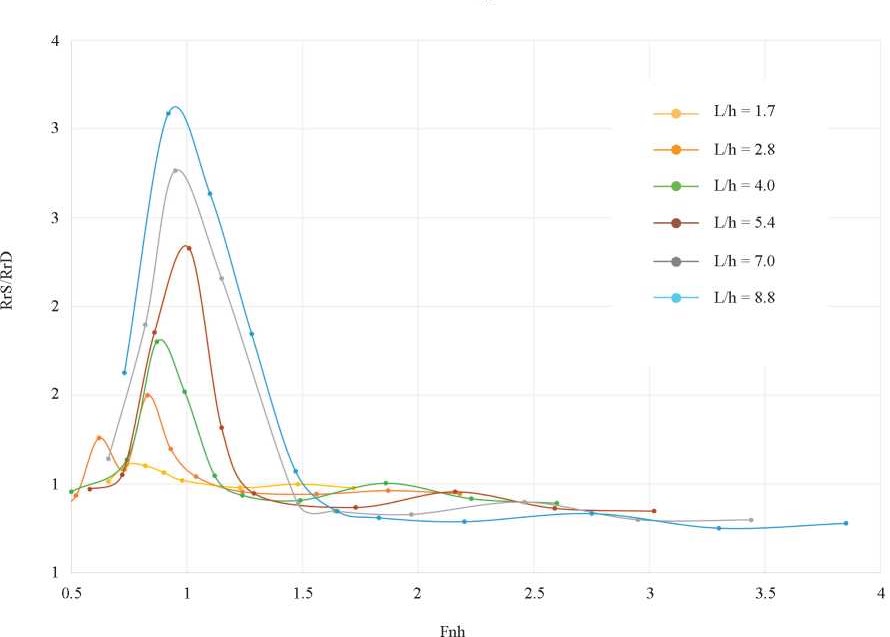
Normally the characteristic wave pattern or Kelvin wave pattern is known; this pattern consists of two groups of waves, the divergent and the transverse. The angle of the diverging bow waves is known with a value of 19°28', however this pattern is only valid for bodies sailing in deep and shallow waters with a number of FF < 0.4 as shown in the Fig. 10. It nh is of great importance to analyze the wave pattern considering that the greatest impact on the drag is on the residual drag as mentioned above.
Fig. 10. Wave pattern Fnh = 0.4.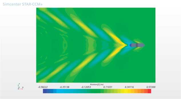
This angle tends to increase as the F numbernh increases to a value of approximately 1.0, reaching angles up to 90° in which the waves appear to be traveling along with the hull. At this point all the energy is contained in the crest of the wave moving at the same speed of the vessel, observing only the transverse waves as shown in Fig. 11 [3].
Fig. 11. Wave pattern Fnh = 0.9.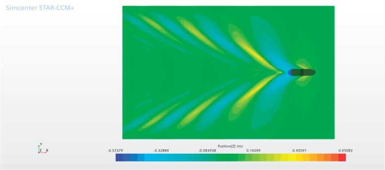
When the Fnh number is greater than 1, the angle of the diverging waves decreases considerably and transverse waves are not visible as shown in Fig. 12.
Fig. 12. Wave pattern Fnh = 1.91.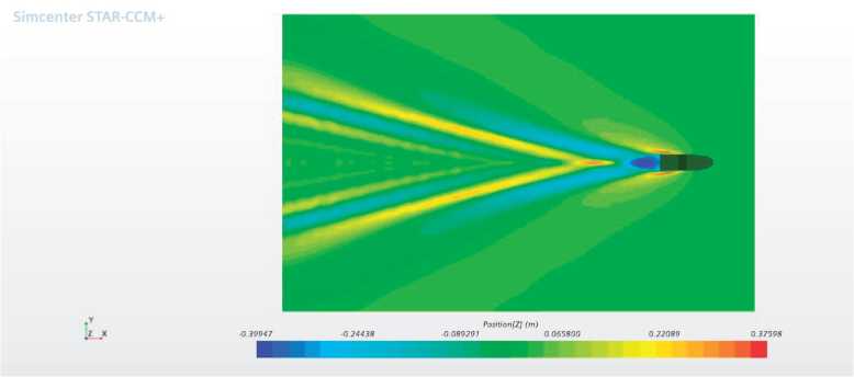
[1] A. I TORO, Shallow- water Performance of a Planning Boat, Annual Meeting of Southeast Section of SNAME, Abril, 1969.
[2] International Towing Tank Conference, ITTC Recommended procedures and Guidelines “Practical Applications for CFD Applications, 2011.
[3] D. RADOJCIC, J. BOWLES, On High Speed Monohulls in Shallow Water, The Second Chesapeake Power Boat Symposium, March, 2010.
[4] A. MILLWARD, M.G BEVAN, Effect of Shallow Water on a Mathematical Hull at High Subcritical and Supercritical Speeds, Journal of Ship Research, Vol 30, No 2, June, 1986.
[5] Comisión Colombiana del Oceano CCO Mapa Esquemático de Colombia URL: https://cco.gov.co/MAPA-ESQUEMATICO.HTML,(seen: 04/05/2021).
[6] Numeca International AB, Documentation guide Fine Marine v8.2, 2007,Brussels,BELGIUM.