Ship Science & Technology - Vol. 15 - n.° 30 - (15-25) January 2022 - Cartagena (Colombia)
DOI: https://doi.org/10.25043/19098642.225
Laura María Núñez Álvarez 1
Juan Camilo Urbano Gómez 1
Juan Pablo Giraldo Grajales 1
Andrés David Wagner Arenas 1
Obed Pantoja Hernández 1
José Mauricio Jaramillo Pulgarín 1
Johan Gerardo Morales Barbosa 1
Daniel Padierna Vanegas 2
1 Universidad Nacional de Colombia, Facultad de Minas, Semillero de investigación Hydrómetra: Movilidad Sostenible, Medellín, Colombia. Emails: lamnunezal@unal.edu.co; jurbanog@unal.edu.co; jupgiraldogr@unal.edu.co; adwagnera@unal.edu.co; ; opantojah@unal.edu.co; jmjaramillopu@unal.edu.co; jgmoralesba@unal.edu.co
2 Universidad Nacional de Colombia, Facultad de Minas, Grupo de Investigación en Procesos Dinámicos-Kalman, Medellín, Colombia. Email: dpadiernav@unal.edu.co
Date Received: July 10th, 2021 - Fecha de recepción: 10 de julio del 2021
Date Accepted: September 21st, 2021 - Fecha de aceptación: 21 de septiembre del 2021
The objective of this research is to provide a tool that allows to quantify the power requirements, energy consumption and the efficiency of the propulsion system of a catamaran with two degrees of freedom according to its speed. Furthermore, it seeks to improve the design process from a phenomenological perspective that gives rise to a better reliability of the result. To achieve this, an electromechanical model is being developed by using the methodology for obtaining phenomenological-based semi-physical models. This model couples the dynamics of a geometry-known ship with its propulsion system, which is constituted by a propeller and a brushless direct current (BLDC) electric motor; at the same time, it uses data from computational simulations related to the hydrodynamics of the submerged components. Finally, the results of using the model with parameters of a specific catamaran and motor are presented. This model allows to properly couple the dynamics of a boat with two degrees of freedom.
Key words: electromechanical model, catamaran, energy consumption, boat design, phenomenological modeling.
El objetivo del trabajo es proporcionar una herramienta que permita cuantificar los requerimientos de potencia, consumo energético y eficiencia del sistema de propulsión de un catamarán con dos grados de libertad según su velocidad. Asimismo, se busca perfeccionar el proceso de diseño desde una perspectiva fenomenológica que dé lugar a una mayor confiabilidad del resultado. Para ello, se desarrolla un modelo electromecánico usando la metodología para la obtención de modelos semi físicos de base fenomenológica. Este modelo acopla la dinámica de una embarcación de geometría conocida con su sistema de propulsión, constituido por una hélice y un motor eléctrico de corriente continua sin escobillas (BLDC); a su vez, utiliza para su construcción datos provenientes de simulaciones computacionales referentes a la hidrodinámica de los componentes sumergidos. Finalmente, se presentan los resultados del modelo tomando parámetros de un catamarán y motor específicos. Este modelo permite acoplar de manera adecuada la dinámica de una embarcación con dos grados de libertad.
Palabras claves: modelo electromecánico, catamarán, consumo energético, diseño de embarcaciones, modelamiento fenomenológico.
Prediction and analysis of Hydrodynamic ship forces are important elements in naval design to determine the vessel hulls and their required propulsor. These forces allow to evaluate both water and air resistance to the ship’s movement and to stablish the consequent propulsion system used to drive the craft [1]. However, resistance and propulsion are interdependent, and their phenomenological interaction behave as a coupled dynamical system. Achieving a system approach, given the objective to get an overall high efficiency of the vessel during its operation, represents an optimization problem [2]. This analysis is plenty complex for most naval architects, even with the current computational capacity [3]. To solve that, a systematic and iterative approach is chosen, as the spiral design process, where design is carried out step-by-step and the ship is split in different subsystems with established relations [3], [4]. This methodology reduces the required time in ship design but increases the later budget estimate for building and operation stage.
To compensate this effect, precise and efficient new methods, and models have been of interest in naval engineering and have been developed throughout the last years to improve design process. For example, dynamical models are well known tools that allow tracking physical phenomena during the ship’s movement, which differ from common static models' scope that are used in design stages [5]. Thereby a dynamical model that accurately represents the physical interactions in a ship can be suitable to get corrective feedback in the subsystems design. As a result, it can improve their capacities, such as ship’s energy efficiency, resistance, stability, and maneuvering [6]-[8]. And it can be used in the previous verification of the ship’s requirements to achieve any possible reduction in building costs and a more reliable model’s feedback for getting the final design.
Various authors have focused their efforts on the dynamic model development of different ships. The reviewed literature shows important improves for getting those models for naval designing and automatic control. The observed results on literature demonstrate a good approximation between the mathematical models and real data of the ship movement [9]-[11]. However, the coupling between the propulsion system and ship dynamics only has been studied in the last years. Some authors have considered the ship movement as load and focused on the modelling of the hybrid propulsion system. This approach avoids the use of ship dynamics and minimizes the motor dynamics [6], [12]. Other authors interpret the coupling between ship and propulsion as an input of the first over the second. For example, [13] models the load torque as a function of the propeller velocity coupled in the rotor propulsor. The most interesting approach is to considerer both dynamics and propose constitutive equations for guaranteeing a robust coupling on the model. Some modeled systems with this approach include coupling among synchronous machine, propeller, and hull [7] and coupling between mobile propulsor and the ship dynamics [5]. However, the current models do not include couplings between the hull dynamics and propulsion system based on brushless direct current motors (BLDC). In Addition, few articles considerer previous result of static models as input for the model development.
This paper proposes a coupled dynamic model constituted by the hydrodynamic forces involved in both ship resistance and propulsion, as well as their effects related to the power system behavior. In this way, it is developed a tool capable to measure the energy requirements by the ship throughout its entire operation. The methodology used in the present work is based phenomenological semi-physical modelling. It is feed by empirical formulations based on constitutive equations of the Process Systems (PS) added to a physical phenomenon developed with momentum balances [14]. Then, the results obtained can be included inside design process to improve ship efficiency. The paper is organized as: Process description is made based on the hull geometry and the motor properties of the vessel designed for testing the model. Detail level is described for getting requirements to achieve the model objective. Modeling Hypothesis are shown the physical and mathematical assumptions made according to the detail level. Process systems are developed conceptual stages of the whole system.
Governing equations are formulated based on the ship electromechanical behavior. Constitutive equations are derived from previous ones to stablish algebraic relations between subsystems. System’s model is pointed out the differential equations that constitutes the model. Simulation is presented the results after running the model. Finally, conclusions are made, and future applications are mentioned.
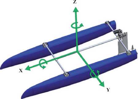
The vessel to model in this paper belongs to the catamaran category. These have two parallel hulls identical in size and geometry (Fig. 1). This architecture provides several advantages over traditional designs, like more stability. The catamaran to model has the following dimensions:
Additionally, it can reach a maximum speed of 5.6 m/s.
The catamaran is thrusted by a brushless DC motor of 5 kW power through a 48V supply. The main reasons why this motor is a good choice as a supply system are its high energy efficiency, high torque capacity and low torque variability when the revolutions per minute (RPM) are modified, compared to other motors like the Brushless AC [15]. In the shaft’s motor, a 4 bladed propeller DTMB4148 is coupled, whose diameter is 30 cm, which provides the necessary thrust to move the vessel. Lastly, there is a rudder NACA 0018 of 60 cm length.
A vessel presents six degrees of freedom (DOF) in a three-dimensional system reference, three corresponding to linear motion and three to rotation (Fig. 1).
Fixed pitch: the pitch angle theta is fixed to a value which corresponds to the angular position of the boat at cruising speed. This angle is not variable, since we recreate the conditions, in which the drag measurements and the propeller performance curves were obtained. For this, the structural support is represented with two components: a spring with an associated force (FK) and a linear damper with dissipative force (FA).
Simplified 2D model: the system moves along two linear directions in the XZ plane, since the other DOF are restricted by the structural support. This happens if it is assumed that the two hulls are moving symmetrically, thus it is not necessary to analyze each hull’s motion independently.
Buoyant Force: The Buoyant Force (FB) is considered as the buoyancy over the group of submerged elements. It depends on the volume that the submerged body occupies, which varies according to the draft c. This draft c is a function of the z position.
Drag Force: the forces associated to drag in the whole submerged volume are the forces due to rudder drag (FAT) and due to hull drag (FAC), which are modeled as non-linear hydraulic dampers. FAT depends on the surge speed; on the other hand, FAC is a piecewise function composed by two sections, which depends on the surge speed as well as the draft.
Propulsion Force: propulsion force (FP) and propeller load torque (Tl), are considered as functions of the advance number (Js), that depends on the propeller angular velocity and the surge speed. The values (required) for these (from which the) regressions are obtained from the theoretical performance curves of the selected propeller (Fig. 2). In the figure, KT refers to the thrust coefficient, KQ to the torque coefficient and EFFY to the mechanical efficiency.
Fig. 2. Theoretical performance values of a propeller.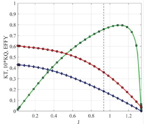
Added Mass: the added mass factor is quantified for the surge acceleration, considering the hull volume that interacts directly with the fluid as explained on [8].
These are the conceptual stages of the process that allow a better comprehension of the whole system. In general, there are two systems: mechanical and power system, each one with its respective subsystems.
Mechanical system: The boat hulls, the propulsion system and the rudder make up the mechanical system, these parts are the ones which interact directly with the water. In dynamic models of boats, two reference frames are found: one that is fixed to the boat located in its center of gravity (CG) and an earth-fixed frame aligned with the water level. In this model, there is a fixed angular position θ in between the two frames. This angle corresponds to the invariable trim of the catamaran.
Fig. 3a shows the general free body diagram without applying the hypothesis we already mentioned, the different subsystems of the mechanical system can be identified. However, for the general equations presented in this paper, a simplified free body diagram is used (Fig. 3b).
Fig. 3. a). Free body diagram of mechanic system without applying the modelling hypothesis. (b) Free body F diagram of mechanic system applying the modelling hypothesis.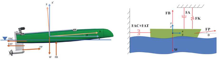
Power system: this system is integrated by a three-phase Brushless DC motor (BLDC) that divides the input voltage in a three-phase AC signal that feeds the three lines of the motor. Fig. 4 shows the equivalent circuit of this BLDC motor.
Fig. 4. Equivalent circuit of BLDC motor [16].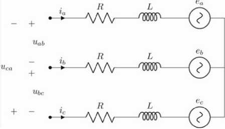
Fig. 5 and 6 illustrate the interaction between these systems. There is an input voltage applied to the motor to generate electric power and finally obtain position values in Z axis and velocities in X and Z. The variables that relate these two systems are: angular velocity and load torque that belongs to the rotational dynamic of the motorpropeller coupling.
Fig. 5. Block diagram of the system.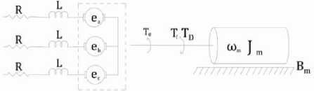
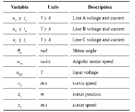
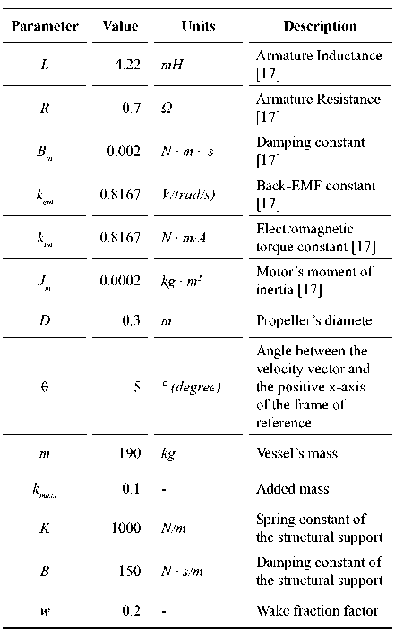
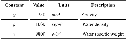
To obtain the equations that describe the electromechanical behavior of the vessel, the balances corresponding to each system have been made. Tables 1, 2 and 3 show the variables, parameters, and constants.
Table 1. Model Variables.
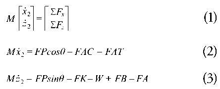
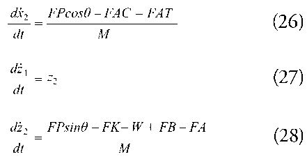
In the mechanical analysis the XZ plane of the vessel is considered, and Newton’s second law is applied to describe the movement kinetics (Equations 1, 2 and 3). Notice that M, defined as M = m(1+kmass), is the ship’s total mass and includes the added mass.
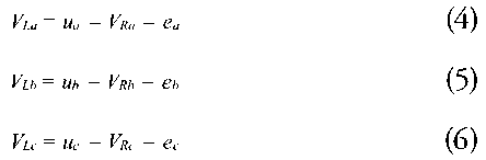
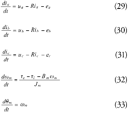
Equations 4, 5, 6 show the result of applying Kirchhoff’s voltage law to each line in the three-phase motor equivalent circuit (Fig. 4).
Finally, the coupling of electrical and mechanical systems can be modelled by following Newton’s second law for rotational dynamics on the shaft where motor and propeller are placed (Equation 7).

To find conclusive results from the governing equations, constitutive equations of the system’s elements are introduced.
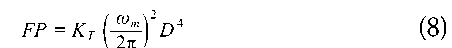
FP is a resultant force from a pressure field generated by the propeller blades in the fluid which has a hydrodynamic profile. In particular, Equation 8 is obtained from a dimensional analysis that allows to relate this force with a coefficient called KT.
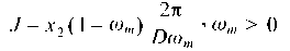
KT coefficient was defined in Modeling Hypothesis and is related to the advanced number J, that is zero when ωm=0. J is defined as
Equation 9, that constitutes FAC, is considered the total resistance whose values for this case are obtained by computational tools, varying the linear velocity x_2 and draft c (Equation 10).
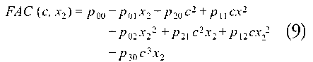

Table 4 shows the values of the coefficients.
Table 4. Parameters of FAC.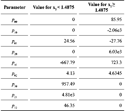
For FAT, the resistance corresponds to a theoretical drag force of the rudder (Equation 11) considered as a submerged element, whose cross section equals a hydrodynamic profile with a known drag coefficient.

FB is governed by the Archimedes’ principle and according to the third modeling hypothesis, the displacement is obtained as a function of the draft. This represents a quadratic regression for the submerged volume of the boat according to its draft. This expression is multiplied by the specific weight γ of water (Equation 12).

W is the weight of the catamaran.

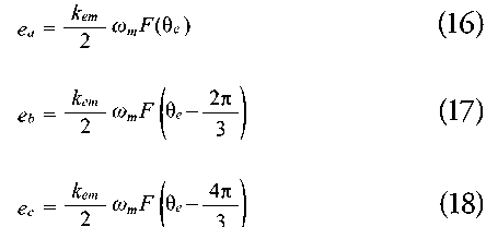
The fixed structural support consists of a damper and a spring, which constitutive equation is defined based on Hooke’s law (Equations 14 and 15).
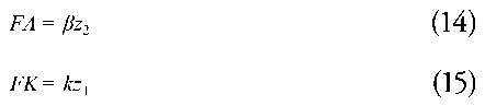
Equations 16, 17, and 18 are the result of applying the Lenz law to obtain the induced voltages in each line.
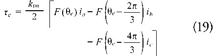
The electrical torque τe is generated by the induced forces on the rotor and it is the result of the sum of the torques in each phase (Equation 19). This is explained by Biot-Savart law.
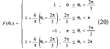
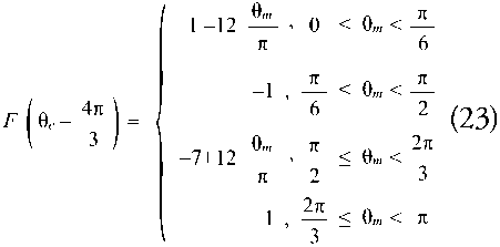
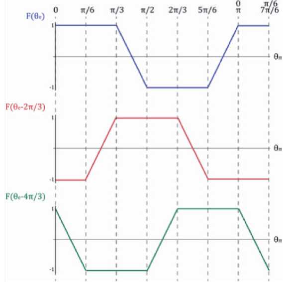
F (θe) is a trapezoidal, periodical, and piecewise function that depends on the electrical angle.
Equation 20 represents each 2π period of F (θe).
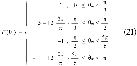
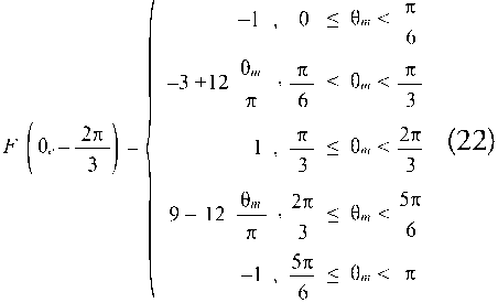
The electrical angle θe is related to the mechanical angle with the expression θe=p/2 θm where p is equal to the number of poles of the motor. In case of a four poles motor, as in this model, Equations 16-19 can be expressed in relation to the angle θm and describing the commutation that occurs in the inverter (Equations 21-23). Fig. 7 is a graphic representation of these functions.
Moreover, the commutation in the inverter must be done in a way that satisfies the conditions for ua, ub and ub depending on the angle θm (Table 5).
Table 5. Voltage value in each phase according to clockwise rotation.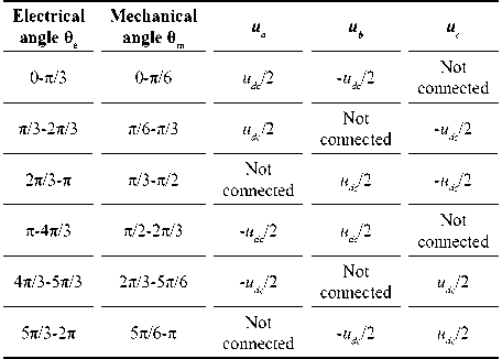
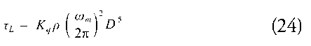
τL corresponds to the load torque of the propeller (Equation 24). This one, is obtained from a dimensional analysis like FP term above mentioned. Likewise, the torque coefficient KQ was defined in Modelling Hypothesis.
τD is the torque that corresponds to the viscous friction of the motor shaft and its direction is opposite to the sense of rotation of the shaft (Equation 25).

The previous equations, constants and parameters were programmed in MATLAB to solve the system of ordinary differential equations (Fig. 8). The input voltage is an input for the model, and it is chosen according to the desired speed profile, including positive and negative acceleration.
Fig. 8. System simulation.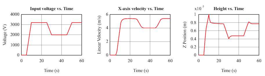
It can be observed that the vessel’s translational speed has a growing behavior until it stabilizes, consequent to the input voltage that the motor receives. Besides, due to the restrictions imposed in the structural support and before the vertical position stabilizes, there are some peaks smaller than one millimeter in very short periods of time. It is evident as well that there is positive acceleration when the voltage increases, and the vessel tends to increase its position in the Z axis. Analogously occurs when the acceleration is negative.
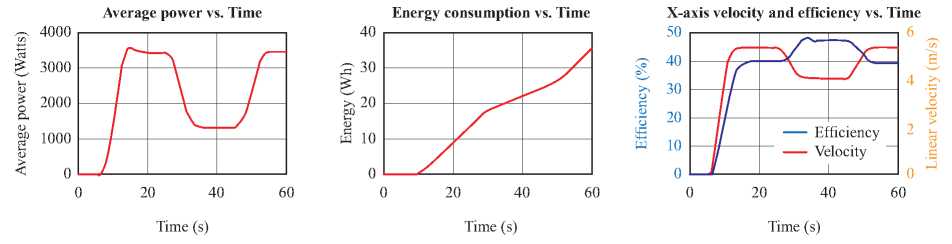
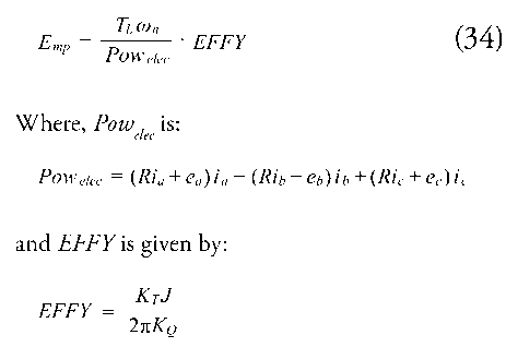
With this information, the motor’s average power is obtained over time. This information would be useful when the real values are required according to the voltage input and the speed variation. In this case, it would be necessary a 3500 watts power to get a 5.4 m/s velocity. After integrating the area under the power’s curve, it is possible to find out the total energy consumption behind a speed routine. As a result, the motor-propeller efficiency (Equation 34) is invariant in steady state and reaches its maximum efficiency when it stabilizes at the smallest speed. That is related with the behavior of FAC: if the vessel’s speed is increased, the required power grows exponentially.
It is shown that the developed model has accurate responses to the variation of the voltage of vessels with electrical propulsion. Now, it can be considered as a tool for the energy consumption evaluation, and if is required, the speed and motion range in which the catamaran is going to move.
During the design phases, the calculation of energy consumption has an important role in the economic and environmental aspects.
The greatest contribution of the model is to provide a tool that allows the verification of parameters evaluated in the vessel design in a more precise way in comparison to the traditional method. For example, the values of consumption are generally obtained in points of specific operation that do not describe in an explicit way, the craft behavior.
Considering the initial considerations and simplifications of the model, for an industrial application it is imperative to reduce the restrictions. Consequently, it is important to increase the degrees of freedom and obtain a model with high reliability for future work.
[1] A. F. MOLLAND, S. R. TURNOCK, AND D. A. HUDSON, “Propulsive Power,” in Ship Resistance and Propulsion: Practical Estimation of Ship Propulsive Power, 2nd ed., Cambridge University Press, 2017, pp. 7-11.
[2] L. BIRK, “Ship Hydrodynamics,” in Fundamentals of Ship Hydrodynamics, John Wiley & Sons, Ltd, 2019, pp. 1-9.
[3] E. C. TUPPER, “Introduction to Naval Architecture,” Fifth Edition., Oxford: Butterworth-Heinemann, 2013.
[4] V. BERTRAM, “Chapter 3 - Resistance and Propulsion,” in Practical Ship Hydrodynamics (Second Edition), Second Edition., V. Bertram, Ed. Oxford: Butterworth-Heinemann, 2012, pp. 73-141.
[5] M. MARTELLI, I. ALESSIO, M. VIVIANI, M. ALTOSOLE, D. GRASSI, AND C. BONVINO, “A simulation approach for planing boats propulsion and manoeuvrability,” The International Journal of Small Craft Technology, vol. 158, pp. 29-42, Apr. 2016, doi: 10.3940/rina.ijsct.2016.b1.180.
[6] L. BARELLI et al., “Dynamic Modeling of a Hybrid Propulsion System for Tourist Boat,” Energies, vol. 11, no. 10, 2018, doi: 10.3390/en11102592.
[7] H. ABROUGUI, H. BOUAICHA, H. DALLAGI, C. ZAOUI, AND N. SAMIR, “Study and modeling of the electric propulsion system for marine boat,” Apr. 2019, pp. 173180, doi: 10.1109/ASET.2019.871052.
[8] T. I. FOSSEN, Guidance and control of ocean vehicles. Chichester, England: John Wiley & Sons, 1999.
[9] H. MOUSAZADEH et al., “Developing a navigation, guidance and obstacle avoidance algorithm for an Unmanned Surface Vehicle (USV) by algorithms fusion,” Ocean Engineering, vol. 159, pp. 56-65, Apr. 2018, doi: 10.1016/j.oceaneng.2018.04.018.
[10] A. GRM, “Mathematical model for riverboat dynamics,” Shipbuilding, vol. 68, pp. 25-35, Apr. 2017, doi: 10.21278/brod68302.
[11] Z. JI AND Y. HUANG, “Autonomous boat dynamics: How far away is simulation from the high sea?,” Apr. 2017, pp. 1-8, doi: 10.1109/OCEANSE.2017.8084927.
[12] B. KOSSEILA, M. B. CAMARA, AND B. DAKYO, “Transient Power Control for Diesel-Generator Assistance in Electric Boat Applications Using Supercapacitors and Batteries,” IEEE Journal of Emerging and Selected Topics in Power Electronics, vol. PP, p. 1, Apr. 2017, doi: 10.1109/JESTPE.2017.2737828.
[13] M. NOORIZADEH AND N. MESKIN, “Design of small autonomous boat for coursekeeping manuevers,” in 2017 4th International Conference on Control, Decision and Information Technologies (CoDIT), 2017, pp. 908-912, doi: 10.1109/CoDIT.2017.8102712.
[14] H. ALVAREZ, J. GARCIA-TIRADO, AND C. BUILES-MONTANO, “Phenomenological based semi-physical modeling for glucose homeostasis in human body,” in 2017 IEEE 3rd Colombian Conference on Automatic Control, CCAC 2017 - Conference Proceedings, Jan. 2018, vol. 2018-January, pp. 1-7, doi: 10.1109/CCAC.2017.8276471.
[15] M. MIYAMASU AND K. AKATSU, “Efficiency comparison between Brushless dc motor and Brushless AC motor considering driving method and machine design,” in IECON Proceedings (Industrial Electronics Conference), 2011, pp. 1830-1835, doi: 10.1109/IECON.2011.6119584.
[16] M. M. MOMENZADEH, A. F. AHMED, AND A. TOLBA, “Modelling and Simulation of The BLDC Electric Drive System Using SIMULINK/MATLAB for a Hybrid Vehicle,” 2014. Accessed: Apr. 13, 2021. [Online]. Available: https://www.researchgate.net/publication/262933380_Modelling_and_ Simulation_of_The_BLDC_Electric_Drive_ System_Using_SIMULINKMATLAB_ for_a_Hybrid_Vehicle.
[17] N. MURUGANANTHAM AND S. PALANI, “State space modeling and simulation of sensorless permanent magnet BLDC motor,” International Journal of Engineering Science and Technology, vol. 2, no. 10, pp. 5099-5106, Oct. 2010, Accessed: Apr. 13, 2021. [Online]. Available: https://www.researchgate.net/publication/50361161_State_space_modeling_and_simulation_ of_sensorless_permanent_magnet_BLDC_ motor.