Ship Science & Technology - Vol. 14 - n.° 28 - (53-62) January 2021 - Cartagena (Colombia)
DOI: https://doi.org/10.25043/19098642.215
César Augusto Salhua Moreno 1
1 Mechanical Engineering Department, Federal University of Pernambuco. Recife, Pernambuco, Brazil. Email: cesar.salhua@ufpe.br
Date Received: January 3rd 2021 - Fecha de recepción: Enero 3 de 2021
Date Accepted: January 27th 2021 - Fecha de aceptación: Enero 27 de 2021
This paper describes the development of a regular hull meshing code using cubic B-Spline curves. The discretization procedure begins by the definition of B-Spline curves over stations, bow and stern contours of the hull plan lines. Thus, new knots are created applying an equal spaced subdivision procedure on defined B-spline curves. Then, over these equal transversal space knots, longitudinal B-spline curves are defined and subdivided into equally spaced knots, too. Subsequently, new transversal knots are created using the longitudinal equally spaced knots. Finally, the hull mesh is composed by quadrilateral panels formed by these new transversal and longitudinal knots. This procedure is applied in the submerged Wigley hulls Series 60 Cb=0.60. Their mesh volumes are calculated using the divergence theorem, for mesh quality evaluation.
Key words: Cubic B-Spline Curves, Hull Mesh, Quadrilateral Mesh Panel, Divergence Theorem.
El presente artículo describe un código computacional, desarrollado para la elaboración de mallas regulares de cascos utilizando cuvas B-Splines cúbicas. El procedimiento de mallado comienza con la definición de curvas B-Spline, en el sentido transversal del casco, sobre las estaciones y los contornos de la proa y popa de un plano de líneas de forma. Por medio de estas curvas B-Spline es posible la creación de nuevos puntos igualmente espaciados en las regiones donde fueron definidas. Posteriormente, con estos puntos son trazadas curvas B-Spline cúbicas en el sentido longitudinal del casco, las cuales son utilizadas para obtener puntos igualmente espaciados, que permiten la creación de nuevas estaciones. Finalmente, los puntos transversales y longitudinales son utilizados para formar los paneles cuadrilaterales de la malla del casco. Este procedimiento es aplicado en los cascos sumergidos del modelo de casco Wigley y Serie 60 Cb=0.60. Los volumenes de estas mallas son calculados usando el teorema de la divergencia para servir como parametro de control de la calidad de la malla.
Palabras claves: Curvas B-Spline Cúbicas, Malla del Casco, Malla de Paneles Cuadrilaterales, Teorema de la Divergencia.
Traditionally, hull lines are designed manually using flexible wood beams known as splines, which can be fixed with lead weights or ducks for drafting a specific curve. The defined spline curve can be controlled locally or globally by moving ducks, which is useful for fairing. Th is process is necessary to obtain the hull and begin calculations such as hydrostatics, hydrodynamics, stability, structures and ship construction and production. This drafting process has been historically represented by mathematical models. One of the first efforts in this area was the work of Frederik Chapman, who in 1776 used parabolas to represent waterlines and other hull surface curves (Ventura, 1996). In 1915, David Taylor also used mathematical equations for parabolas, hyperbolas and fifth order polynomials to represent the hull shapes of his systematic series. Between 1915 to 1970 several researchers used polynomials and other analytical geometric functions to represent hulls. Nevertheless, parabolas and conventional polynomial equations are difficult when fairing and locally modifying curves.
Mathematical models more similar to the wood spline drafting procedure began to appear. In 1957, Paul de Casteljau developed a spline described by parametric curves defined by control points, to be introduced in the Citroën automotive industry. In a parallel research, Paul Bezier developed an equivalent mathematical representation known as Bezier curve, while he had been working for Renault during 1962. A limitation of these curves was the impossibility to be modified locally for nearby control points, and its dependence on the number of control points with curve degree (Rogers, 1977).
One of the most important contributions to a closer mathematical spline representation, without the issues of the Bezier curves, occurred in 1940, when Schoenberg developed a spline function based on a parametric mathematical representation of third degree polynomial to fit statistical data named as B-Spline or Basis Spline (Cabral, et al., 1990). The properties, characteristics and piecewise adaptation of this function were studied and developed in 1972 by Carl de Boor (De Boor, 2001). Further, B-Splines were introduced into Computer Aided Design (CAD) software by J. Ferguson for Boeing Co in 1963.
With increasing computer processing capacity in the 60's, the application of CAD in ship design also grew. Nowadays it is possible to perform hydrostatic, stability, structural and hydrodynamic analysis with it. Using a group of knots known as a mesh to represent the hull surface. Th is mesh can be composed of quadrilateral (regular) or triangular (irregular) knot arrangements.
This paper describes the mathematical formulation and methodology using in Salhua (2010) for a quadrilateral hull mesh generation code, using cubic B-Splines curves to represent submerged hulls. Finally, the Wigley model Series 60 Cb=0.60 hull are used for mesh generation evaluations.
A B-Spline function is a mathematical representation of a piecewise polynomial curve through parametric equations. Each segment is joined following geometric (C0), slope (C1) and curvature (C2) continuity conditions. Moreover, a cubic B-Spline function has a polynomial order of 4 and has to follow two conditions (Riesenfeld, 1973):
a) The cubic B-Spline needs to be a third degree polynomial on each segment.
b) The first and second derivatives are continuous on each segment.
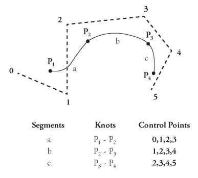
A piecewise cubic B-spline curve can be composed by m segments where each one is defined by four control points. A complete B-Spline curve needs to have m+1 knots and m+3 control points. Each neighboring segment shares three control points, so each segment has a different one, (Yamaguchi, 1978). As a example shown in Fig. 1, the curve has 4 knots, 3 segments and 6 control points.
Fig. 1. Cubic B-Spline with 3 segments.
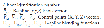
The B-spline mathematical formulation of cubic B-spline knots depends on blending the functions and control points, see equation (1), (Cabral, et al., 1990) and (De Boor, 2001).

Where:
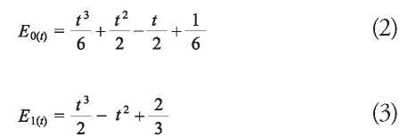
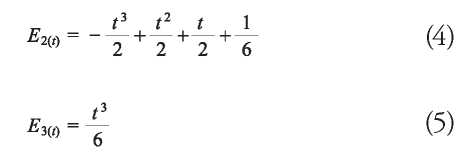
The blending functions are created to transform a polynomial equation into a piecewise and parametric curve B-Spline equation. These are imposed on each segment along curve and satisfy C0, C1, C2 continuity conditions. Primarily, they allow for local control of the curve shapes. That is an improvement against simple polynomials, in which any change in any part modifies the entire curve. They are defined in 1D parameter t and vary from 0 to 1. Therefore t=0 corresponds to the initial knot segment and t=1 corresponds to the last one. The cubic B-Spline blending functions are shown in equations (2) to (5) (Yamaguchi, 1978):
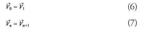
The number of control points exceeds the number of knots, Yamaguchi (1978) suggests the use of two additional boundary conditions equations to complete the system, see equations (6) and (7).
These conditions are applied as shown in Fig. 2.
Fig. 2. Open B-Spline curve.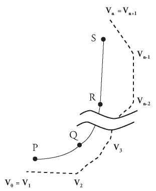
Considering the parametric variable t of the blending B-Spline functions equal to zero to identify the initial knot and one for the final knot of each curve segment, (Cabral, et al., 1990). The base functions are:
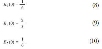
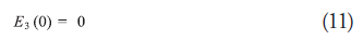
The last base function E3 (0) is equal to zero when t = 0, so the mathematical cubic B-Spline equation can be represented with only three base functions and control points, see equation (12).

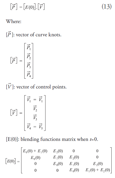
Equation (12) is applied through the four knots of Fig. 1 to obtain B-Spline control points by solving the linear system shown in (13) with the application of boundary conditions shown in equations (6) and (7).
A total length of the B-Spline curve is calculated by each segment curve and then added for a total, see equation (14).
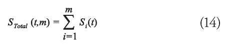
Where:
Si (t): Length of segment i.
t: parameter of blending functions, in this case t = 1.
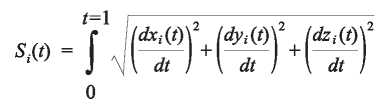
m: Total number of segments of a B-Spline curve. xi , yi , zi : Coordinates of the B-spline curve
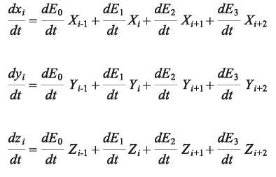
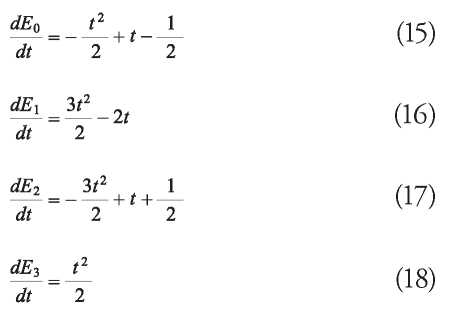
The derivatives of the blending functions are shown as follows:
A hull lines plan is used to extract knots from three regions: Stern contour, Transversal stations and Bow contour, see Fig. 3.
Fig. 3. Hull lines of ship.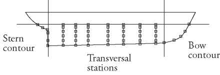
B-Splines curves are defined individually over each station, stern and bow contours. Further, their total lengths are calculated (Stotal ), as described in section 2.2.
Fig. 4. Station divided in equal length subdivision.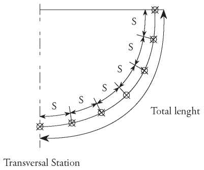
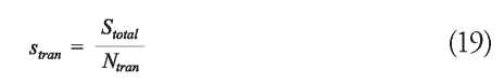
Over each B-Spline curve, the total length is equally subdivided by a desired subdivision N tran , as follows:
To obtain the segments and t parameters in each curve that correspond to the equally spaced length subdivision, see Fig. 5. A root-finding algorithm numerical method is applied for the following function:
Fig. 5. Station equally subdivision.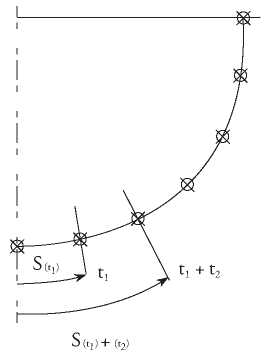
Where:
i: is the segment number of a curve.
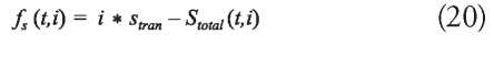
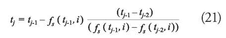
To solve the equation (20), the secant method is used (Nakamura, 1991), see equation (21).
Where:
j: index subdivision of t.
Through this subdivision procedure, new knots are created to obtain equal subdivided B-Spline curves. In these equally spaced knots, longitudinal B-splines curves are defined and subdivided into equally spaced knots (NLong). Furthermore, over these new longitudinal knots, new transversal stations and stern and bow contours are created. This procedure is executed transversally and longitudinally to obtain a new hull discretization.
Through this subdivision procedure, new knots are created to obtain equal subdivided B-Spline curves. In these equally spaced knots, longitudinal B-splines curves are defined and subdivided into equally spaced knots (NLong). Furthermore, over these new longitudinal knots, new transversal stations and stern and bow contours are created. This procedure is executed transversally and longitudinally to obtain a new hull discretization.
The generated mesh is used to define single planar quadrilateral panels, see Fig. 6 , over the entire hull surface.
Fig. 6 Panel configuration.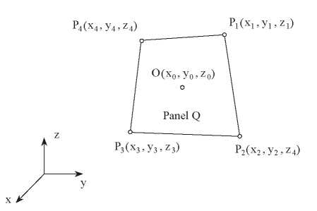
The hull volume is calculated through the transformation of volumetric into superficial integration. Through the divergence theorem, see equation (22), applied over all hull surface.
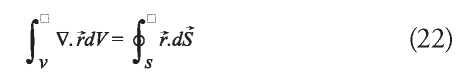
Where:
Position vector 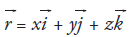
x + y + z :coordinates of each quadrilateral panels.
Considering the hull surface is composed by several planar panels, a formulation for volume calculation is shown in equation (23), (Alvarez & Martins, 2007).
Where:
V: volume (m3).
Xo(Q), Yo(Q), Zo(Q): centroid coordinates of panel Q.
xn(Q), ny(Q), nz(Q): normal vector components in the centroid of panel Q.
NT: total number of hull surface panels.
In order to evaluate the effectiveness of the computer code implemented with the methodology described previously, the Wigley hull (Journee, 2001) Series 60 Cb = 0.6 hull (Todd, 1953) are used for mesh generation tests and their submerged volume is used for mesh quality evaluation.
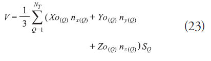
This hull has round shapes and can be represented using a parabolic equation, see equation (24), shown in Journee (2001).
Where:
B: beam.
L: length.
T: draught.
x: longitudinal coordinate of a hull station.
z: vertical coordinate of a hull station.
y: transversal coordinate of a hull station.
The main dimensions of the hull used are:
The submerged hull lines have fore and aft symmetry as follows:
Fig. 7. Submerged Wigley hull lines.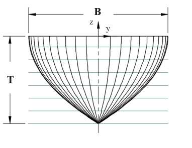
Extracting discrete points of these hull stations as original knots, several meshes are generated only over one band of the hull, due to transversal symmetry. Two of these hull meshes are shown in Fig. 8.
Fig. 8. Wigley Hull with two types of discretization.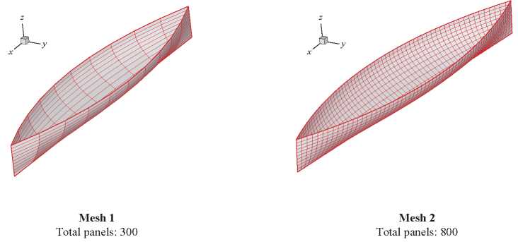
Fig. 9 shows a comparison between the original and B-spline knot stations in longitudinal positions x=0.842m and x=0.526m. The cubic B-spline curves represent properly the behavior of these stations, despite the use few original knots. This is due to the C2 continuity between the original and the B-Spline station.
Fig. 9. Station comparisons between original and B-spline representations.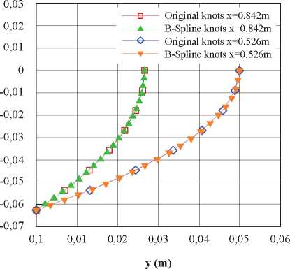
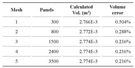
A comparison of several calculated mesh volumes with theoretical value (Table 1), is shown in Table 2. From Table 2, it is possible to observe a good convergence with increasing mesh refinement.
Table 1.Dimensions of Wigley hull.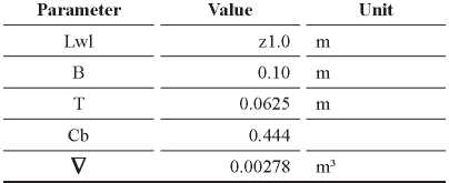
This hull represents a merchant-type ship, its development is described in Todd (1953). It has a flat bottom which is almost ship length and a straight side at the midship region, see submerged body in Fig. 10.
Fig. 10. Series 60 Cb = 0.60 submerged hull lines.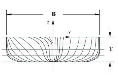
The main dimensions of the submerged body are described in Table 3.
Table 3. Dimensions of Wigley hull.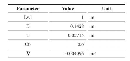
Through the methodology described before, it is possible to create and refine hull meshes, see Fig. 11.
Fig. 11. Series 60 Cb=0.6 Hull with two types of discretization.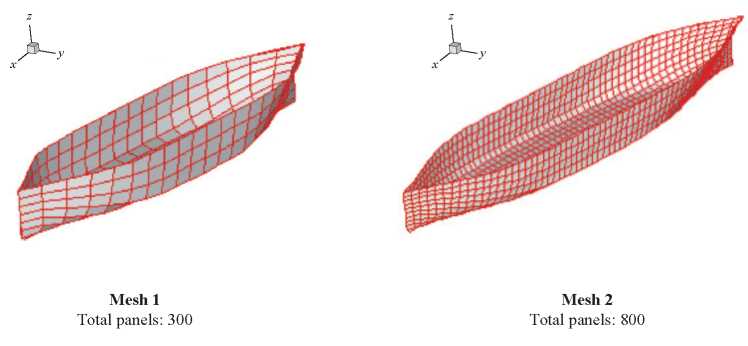
Considering the offset table, described in Todd (1953), as original knots to represent a B-Spline curve, a poor representation of midship section was observed, see Fig. 12. This is due to the discontinuity of the curvature (C2) between straight parts (bottom and side) and the rounded bilge. For that reason, the cubic B-Spline curves used in this work do not represent properly the stations composed by straight and rounded parts.
Fig. 12. Midship station comparisons between original knots and spline representation.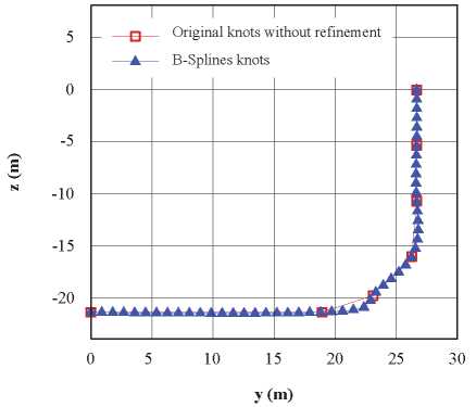
To overcome the issue of C2 continuity, flat bottom and bilge are defined by more original knots. This action increases the number of control points over these parts, adjusting the curvature transition of the B-Spline curve segments more accurately, but the required number of original knots is high, as shown in Fig. 13.
Fig. 13. Midship stations comparisons between original knots and refinement and spline representation.
Table 4 presents a comparison of several calculated mesh volumes with the expected one (Table 3).
Table 4. Comparison of volumes of Series 60 Cb =0.60 meshes.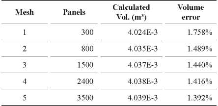
From Table 4, it is possible to see a convergence behavior increasing mesh refinement.
A numerical code for hull mesh discretization requires further development. This code uses cubic B-Spline curves for the representation of transversal stations, bow and stern contours of a curved hull plan lines. This procedure is the initial stage to create new equally spaced knot curves in transversal and longitudinal directions to conform the mesh.
The parameter for the hull mesh evaluation quality is the submerged volume. It is evaluated using the divergence theorem associated with the quadrilateral panels of a hull mesh.
Two hulls are used for code evaluation, Wigley and Series 60 — Cb = 0.60.The Wigley hull has parabolic stations, in which the cubic B-Splines used adjust properly. Several mesh refinements have shown a good convergence even in a coarse mesh. This is due to the hull lines being rounded with C2 continuity and cubic B-Spline.
In the case of the Series 60 — Cb = 0.60 hull, the flat bottom and side of the parallel body creates problems in the cubic B-Spline representation due to C2 discontinuity. To overcome this issue, more original knots need to be allocated in the straight regions to force the cubic B-Spline curves to adjust to these stations. This adjustment allows to work around this limitation. Nevertheless, the value of the volume converges with increasing refinement. That was expected because a higher refinement allows to represent the submerged body more accurately.
To solve discontinuity problems, the use of a B-Spline formulation with non-uniform blending functions and special treatment of control points in the connection between regions as flat bottom or straight side with round bilge, as described in Cabral et al. (1991).
[1] R. L. ALVAREZ and M. R. MARTINS, “Otimização das Formas de Cascos de Deslocamento em Relação a sua Resistência ao Avanço”, in XX Pan-American Conference of Naval Engineering (COPINAVAL), São Paulo, 2007.
[2] CABRAL J., WROBEL L. and BREBBIA C., A BEM formulation using B-splines: II- multiple knots and non-uniform blending functions, Engineering Analysis with Boundary Elements. 1991, vol 7, issue 1.
[3] CABRAL J., WROBEL L. and BREBBIA C., A BEM formulation using B-splines: I- uniform blending functions, Engineering Analysis with Boundary Elements. 1990, vol 7, issue 3.
[4] DE BOOR C., A Practical Guide to Splines, Applied Mathematical Sciences. 2001.
[5] J. J. JOURNEE, “Discrepancies in Hydrodynamic Coefficients of Wigley Hull Forms”, in Proceedings of the 3rd International Conference on Marine Industry (MARIND), Varna, 2001.
[6] S. NAKAMURA, Métodos Numéricos Aplicados com Software. 1th ed. Naucalpan de Juarez, Mexico, Prentice Hall Inc, 1991.
[7] NOWACKI H., Five Decades of Computer-Aided Ship Design, Computer-Aided Design. 2010, vol 42, pp 956-969.
[8] R. F. RIESENFELD, “Applications of B-Spline Approximation to Geometric Problems of Computer Aided Design”, Ph.D. dissertation, Dept. of Systems and Information Science, Syracuse University, NY, 1973.
[9] ROGERS D. F,. “B-Spline Curves and Surfaces for Ship Hull Definition”, in Symposium of Computer Aided Hull Surface Definition (SCAHD), Annapolis, MD, 1973.
[10] C. SALHUA, “Hydrodynamic Interference between Ships with Forward Speed in Waves”, D.Sc. dissertation (in portuguese), Dept. of Naval and Ocean Engineering, Federal University of Rio de Janeiro, RJ, Brazil, 2010.
[11] TODD F.H., Some further experiments on single-screw mechant ships forms - serie 60, SNAME Transaction, 1953.
[12] USHATOV R., POWER H. and Rêgo SILVA J. J., Uniform bicubic B-splines applied to boundary element formulation for 3-D scalar problems, Engineering Analysis with Boundary Elements, 1994, vol 13, pp. 371-381.
[13] VENTURA M. F., “Ship Hull Representation by Non-Uniform Rational B-Spline Surface Patches”, M.Sc. thesis, Dept. of Naval Architecture and Ocean Engineering, Glasgow, UK,1996.
[14] YAMAGUCHI, F. A., A New Curve Fitting Method Using a CRT Computer Display, Comp. Graph and Image Processing. 1978, pp 425-437.