Sandra Carrillo1 y Juan Contreras2,
In this paper we present a method for obtaining a second order Nomoto model that describes the yaw dynamic of a Patrol River Boat. This model is obtained from experimental input and output data gathered from the turning circle maneuver. System identifications techniques and a gray box model are employed to find the coefficients of the Nomoto model. The results of the identification process as well as the results of validation process are presented.
Key words: second order Nomoto model, coefficients of Nomoto, maneuverability, system identification, gray box model.
Este artículo describe la obtención del modelo de Nomoto de segundo orden para una patrullera de apoyo fluvial PAF a partir de datos experimentales, derivados de pruebas estándares de maniobra realizadas en aguas poco profundas. Se utilizan ténicas de identificación de sistemas y un modelo de caja gris que permite extraer los coeficientes del modelo de Nomoto. Se presentan los resultados del proceso de identificación, así como de los procesos de validación utilizando datos de pruebas diferentes a la empleada en la identificación.
Palabras claves: modelo de Nomoto de segundo orden, coeficientes de Nomoto, maniobrabilidad, identificación de sistemas, modelo de caja gris.
According to the International Maritime Organization, IMO, the International Association of IMCA Marine Contractors, and other classes of certification societies, a dynamic positioning vessel is related to the automatic control of the position of the vessel and the course with respect to one or more position references for the use of active propellers [1]. Maintaining the course of a vessel is a complex problem due to the vessel's nonlinear dynamics, but it has a great impact on the economy, safety and operation of vessels [2,3].
For the description of the dynamics of surface vehicles, the authors have used different types of models, such as the Nomoto model [4,5,6], the Norbin model [7] and others.
For the data of the tests the Patrol Boat of Heavy Fluvial Support "PAF-P" of 3rd generation built by COTECMAR 2009 has been taken as a study model. The ship was subjected to the approval of an evolutionary circle at different approach speeds and rudder angles. , zig-zag and emergency stop in shallow water (H / T = 2.4) and deep water (H / T> 10) [8,9].
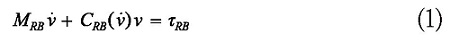
The equations that control the dynamics of a ship are derived from the equations of motion of a rigid body with 6 degrees of freedom. These equations are shown below in vector form [10]:
Where MRB is the mass matrix, CRB is the centripetal and coriolis matrix, v is the angular and linear velocity vector of the rigid body ([u, v, w, p,q, r]T) and tRB is the generalized vector of external forces and moments ( [X, Y, Z, K, M, N]T ).
From equation (1) an expansion of the terms of the 6 degrees of freedom is made [10]:
Where X, Y, Z are external and hydrodynamic disturbing forces and K, M and N are hydrodynamic and external disturbance moments.
To simplify this model of equations of six degrees of freedom to 3 degrees, the following assumptions are made:
This produces three simplified nonlinear equations:
The disturbed equations of motion are based on an additional assumption:
• The speed of deviation (sway) v, and the yaw rate r and the rudder angle δ are small.
This implies that the mode of advance (surge) can be dissociated from the yaw and deflection modes assuming that the average speed of advance u0 is constant for a constant thrust. In the same way, it is assumed that the average yaw and yaw velocities are v0 = r0 = 0 . As such:
Where Δu, Δv and Δr are small disturbances of nominal values u0 v0 and r0 , and ΔX, ΔY and ΔZ are small disturbances of nominal values X0, Y0 and N0.
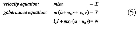
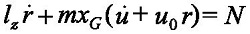
Assuming that higher order disturbances can be neglected, the nonlinear equations of motion can be expressed as:
Note that the governing equations of motion are completely decoupled from the velocity equation.
The assumption that the average forward speed is constant implies that this model is only valid for small rudder angles.
First-order Nomoto equation
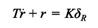
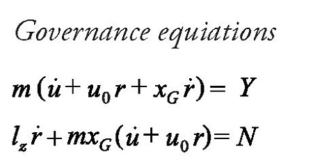
Starting from the governance equation:
Reorganizing and replacing the governance time constant T = lz / mxGu0 and the rudder gain K = N / δRmxGu0 would be expressed as the First Order Nomoto Equation of the form [11]:
Or alternatively:
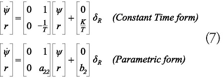
Reorganized the equation to the state-space form x = Ax + Bu y y = Cx, The First Order Nomoto model becomes:
Second order Nomoto equation
A second-order deviation-yaw model is obtained from the motion equations with 3 degrees of freedom and uncoupled in advance, assuming small perturbations we have:
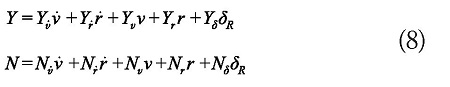
Assuming the origin in the center of gravity (xG = 0). The linear theory suggests that hydrodynamic force and momentum can be modeled as (Davidson and Schiff, 1946) [12]:
Therefore, we can write the equations of motion in the form of state-space according to:
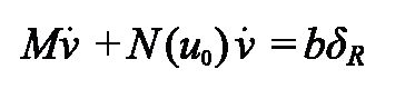
and the Nomoto model is obtained:
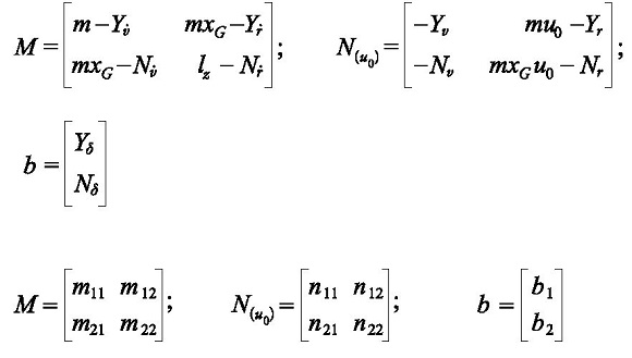
Where v = [v,r]T is the state vector, δR the rudder
angle, and:
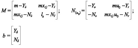
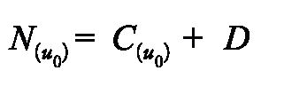
The N(u0) matrix is obtained by the is obtained by the linear sum of the damping D and the terms of Coriolis C(u0) and centripetal (additional terms mu0 and mxGu0), which means:
The corresponding space-state model is obtained, leaving v = [v,r]T is the state vector and u = δR.
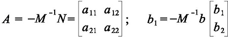
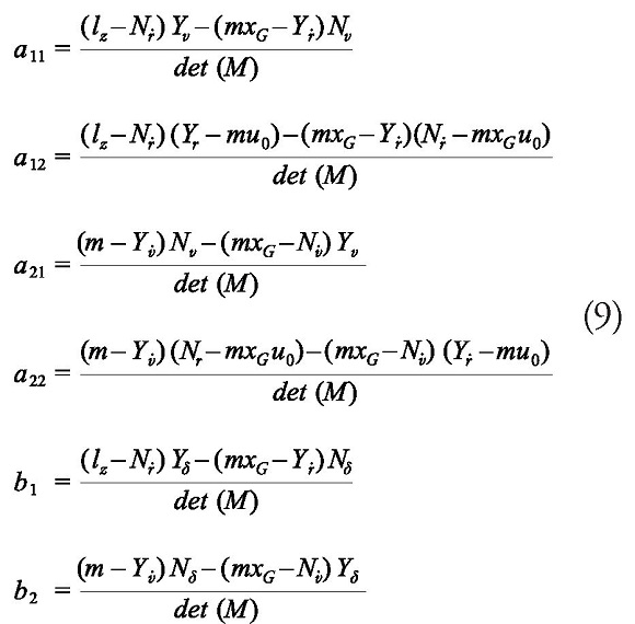
with:
The coefficients are defined as [13]:
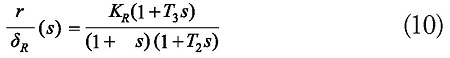
These models are obtained by eliminating the deviation speed from Mv + N (u0)v = bδR to get the Nomoto transfer function between r and δR , which is:
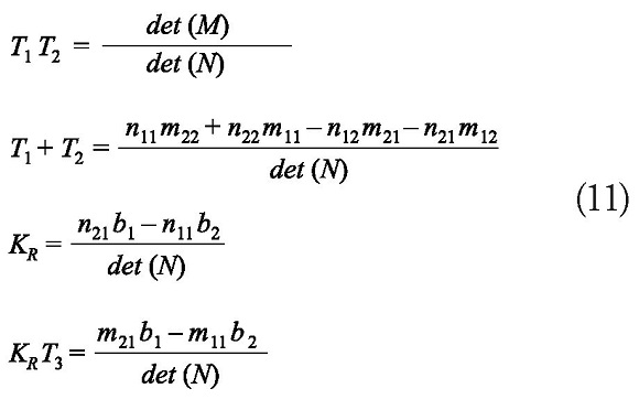
The parameters of the transfer function are the relationships with hydrodynamic derivatives such as:
Where the elements nij , mij and bi are defined as:
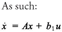
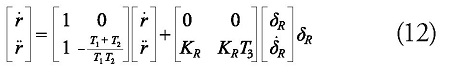
Expressing the equation x= Ax + b1u, it becomes
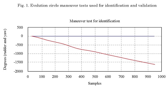
To obtain a simplified mathematical model (under order) that represents the dynamics in an approximate way, identification techniques were used. In the process of identification and validation of the model that describes the dynamics of the vehicle under study in the horizontal plane, several tests were performed based on the maneuver test of the evolutionary circle. Two (2) of these tests can be seen in Fig. 1 The rudder angle is considered as input and the heading angle as an output.
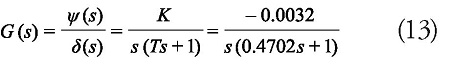
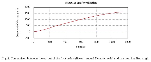
It was used, as a second identification technique, the use of the method of least squares using as input the rudder angle and as output the variation of the angle of course (yaw rate), in order to achieve a gray box model that would allow to associate the parameters with the coefficients or indices of a first order Nomoto model. The obtained coefficients are: K = -0.0032 and T = 0.4702, with which the first-order Nomoto model is expressed by
Fig. 2 shows the output, or heading angle, generated by the first-order Nomoto model compared to the actual heading angle. The standardized mean squared error was 0.2883.
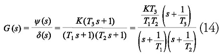
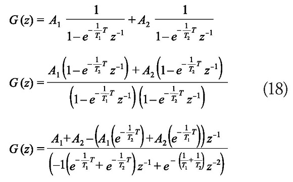
The second-order Nomoto model is given by the expression:
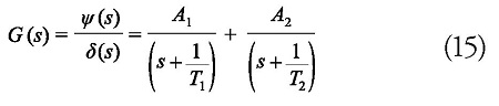
If we break down by partial fractions, we have to
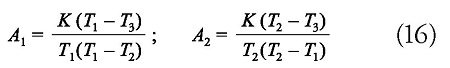
With which the following is obtained
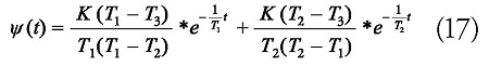
That is, the response in the time domain will be given by
Then, in the Z domain
Where T is the sampling time.
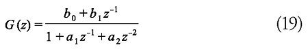
If we make an analogy with a discrete second-order model expressed by the following equation:
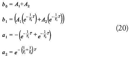
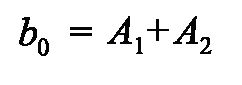
We have that:
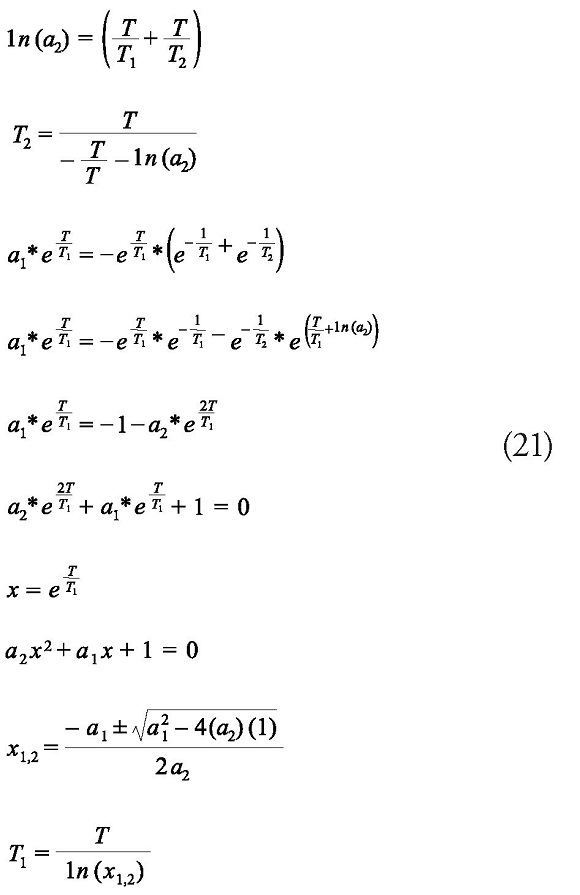
Where we get:
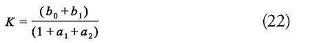
We calculate K it from the gain of the model in discrete time (z = 1), as follows:
Finally we find T3, as follows:
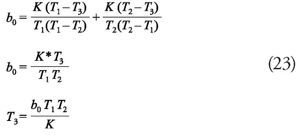
The coefficients obtained are: K = -0.1724, T1 = 2.0875, T2 = 0.3179 and T3 = 0.1830, with which the second-order Nomoto model is expressed by
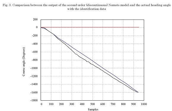
Fig. 3 shows the output, or heading angle, generated by the second-order Nomoto model compared to the actual heading angle. The standardized mean square error obtained was 0.0397.
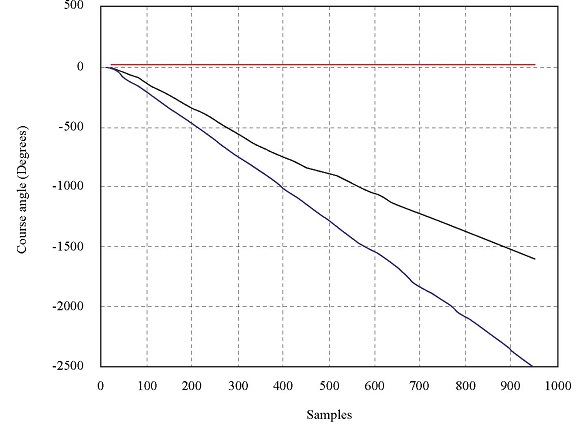
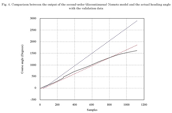
Fig. 4 shows the output, or heading angle, generated by the first and second order Nomoto models compared to the actual heading angle in the validation exercise. The standardized mean square error obtained with the first order Nomoto model was 0.3826, while with the second order Nomoto model it was 0.0516.
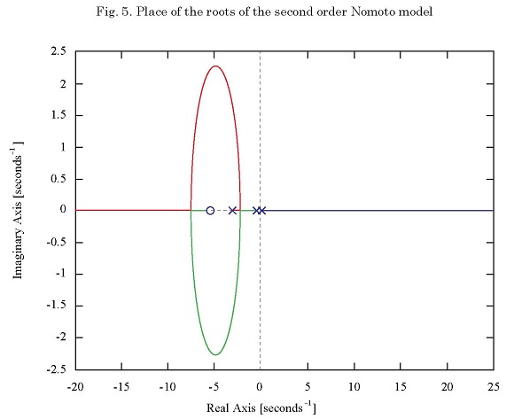
Fig. 5 shows the place of the roots of the second order Nomoto model. Three poles are observed: two of them are located on the left side of the plane S, which remains on the negative real axis for system gain levels less than 23.6; the other pole is located at the origin and moves to the right if the gain is incremented, which would generate system instability. This pole located in the origin is the one that generates the movement of evolutionary circle for the entrance (change in the rudder) type step.
A methodology was presented to obtain the order Nomoto model of a PAF fluvial support patrol using identification technique and using experimental data from a standard such as the turning circle maneuver. The mathematical model order Nomoto model of a PAF fluvial support obtained presents a standardized mean square error of 0.0397 in the identification process and 0.0516 in the validation process, which shows a fairly high approximation. The test used for validation was done with a turn to port while the one used for identification was made to starboard.
The analysis of the place of the roots of the Second Order Nomoto model shows the temporal behavior of the system. The pole located at the origin is the one that causes an indefinite turn to port, or starboard, since its location at the origin of the S plane implies an unstable or critically stable behavior.
The authors thank Dr. VALM Jorge Enrique Carreño Moreno, who provided important knowledge to carry out the development of this project.
[1] WANG MENG, LI HONG SHENG, MIAO QING and BIAN GUANG RONG. “Intelligent control algorithm for ship dynamic positioning”. Archives of Control Sciences, Vol. 24, No. 4, p.p.: 479-497. 2014.
[2] HAIJUN XU, WEI LI, YANG YU and YONG LIU. “A Novel Adaptive Neural Control Scheme for Uncertain Ship Coursekeeping System”. Sensors & Transducers, Vol. 178, No. 9, p.p.: 282-285, 2014.
[3] SK. SHARMA, W. NAEEM, R. SUTTON. “An Autopilot Based on a Local Control Network Design for an Unmanned Surface Vehicle”. The Journal of Navigation. Vol. 65, p.p.: 281-301. 2012.
[4] VELASCO, F.J., REVESTIDO, E., LÓPEZ, E., MOYANO, E., HARO CASADO, M. “Autopilot and Track-Keeping Simulation of an Autonomous In-scale Fast-ferry Model”. 12th WSEAS International Conference on Systems, Heraklion, Greece, July 22-24, 2008.
[5] VELASCO, F.J., REVESTIDO, E., LÓPEZ, E., MOYANO, E., HARO CASADO, M. “Simulation of an Autonomous In-scale Fast-ferry Model”. International Journal of System Applications, Engineering and Development , Vol. 2, No.3, p.p.: 114-121. 2008.
[6] BANAZADEH A, GHORBANI MT. Frequency domain identification of the Nomotomodel to facilitate Kalman filter estimation and PID heading control of a patrolvessel. Ocean Eng 2013;72:344-55.
[7] AULIA ZITI AISJAH, An Analysis Nomoto Gain and Norbin Parameter on Ship Turning Maneuver , IPTEK, The Journal for Technology and Science, Vol. 21, No. 2, May 2010.
[8] CARREÑO, J. E., “Simulación de maniobras de buques con sistemas de propulsión no convencional en aguas poco profundas”, Madrid, España: Universidad Politécnica de Madrid, Tesis doctoral, 2012.
[9] CARREÑO, J. E., MORA, J. D., PÉREZ, F. L., “Mathematical model for maneuverability of a riverine support patrol vessel with a pump-jet propulsion system”, Ocean Engineering, Vol. 63, 2013, pp. 96-104
[10 ] T. I. FOSSEN, Guidance and Control of Ocean Vehicles, John Wiley and Sons,New York, 1994.
[11] TZENG, C., and CHEN, J., “Fundamental Properties of Linear Ship Steering Dynamic Models,” Journal of Marine Science and Technology, Vol. 7, No. 2, pp 79-88, 1999.
[12] REVESTIDO E., VELASCO F., LÓPEZ E., Diseño de Experimentos para la Estimación de Parámetros de Modelos de Maniobra Lineales de Buques. Elsevier Revista Iberoamericana de Automática e Informática industrial 9 (2012) 123-134.
[13] POLLAND, S. Recursive parameter identification for estimating and displaying Maneuvering vessel path, Thesis 2003.