Ship Science & Technology 10(20): 31-40, 2017
Hassan Ghassemi1, Sohrab Majdfar2, Hamid Forouzan3.
1 Department of Maritime Engineering, Amirkabir University of Technology, Tehran. Email: iran. gasemi@aut.ac.ir
2 Department of Marine Engineering, Imam Khomeini University, Nowshahr, Iran. Email: sohrabmajd@gmail.com
3 Department of Marine Engineering, Imam Khomeini University, Nowshahr, Iran. Email: hamid.foruzanl348@gmail.com
Date Received: November 29th 2016 - Fecha de recepción: Noviembre 29 de 2016 Date Accepted: December 19th 2016 - Fecha de aceptación: Diciembre 19 de 2016
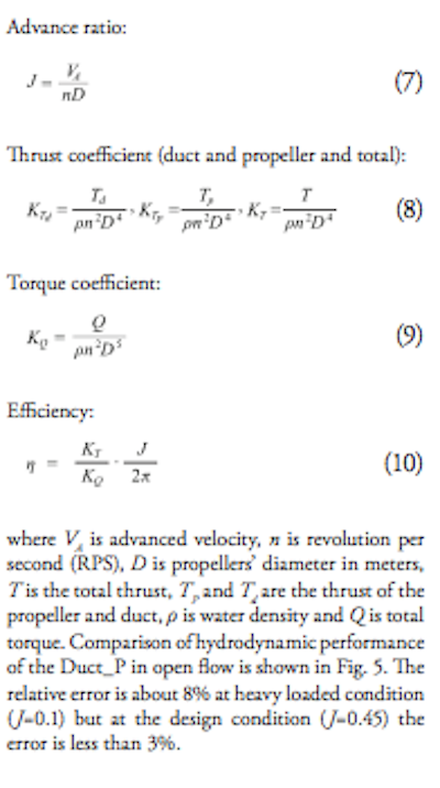
The purpose of this paper is to calculate the hydrodynamic performance of a ducted propeller (hereafter Duct_P) at oblique flows. The numerical code based on the solution of the Reynolds-averaged Navier-Stokes equations (RANSE) applies to the Kaplan propeller with 19A duct. The shear-stress transport (SST)-k-co turbulence model is used for the present results. Open-water hydrodynamic results are compared with experimental data showing a relatively acceptable agreement. Two oblique flow angles selected to analyze in this paper are 10 and 20 degrees. Numerical results of the pressure distribution and hydrodynamic performance are presented and discussed.
Key words: Ducted propeller, Hydrodynamics forces, Oblique flow.
Este trabajo tiene como objetivo calcular el rendimiento hidrodinámico de la hélice canalizada (en lo sucesivo Duct_P) en flujos oblicuos. El código numérico basado en la solución de las ecuaciones de Navier-Stokes promedio de Reynolds (RANSE) se aplica a la hélice Kaplan con conducto 19A. Para los resultados actuales se utiliza el modelo de turbulencia de transporte de esfuerzo cortante (SST) -k-oo. Los resultados hidrodinámicos de aguas abiertas se comparan con datos experimentales que muestran un acuerdo relativamente aceptable. Dos ángulos de flujo oblicuo seleccionados para analizar en este documento son 10 y 20 grados. Se presentan y discuten los resultados numéricos de la distribución de presión y el rendimiento hidrodinámico.
Palabras claves: hélice acodada, fuerzas hidrodinámicas, flujo oblicuo.
Introduction
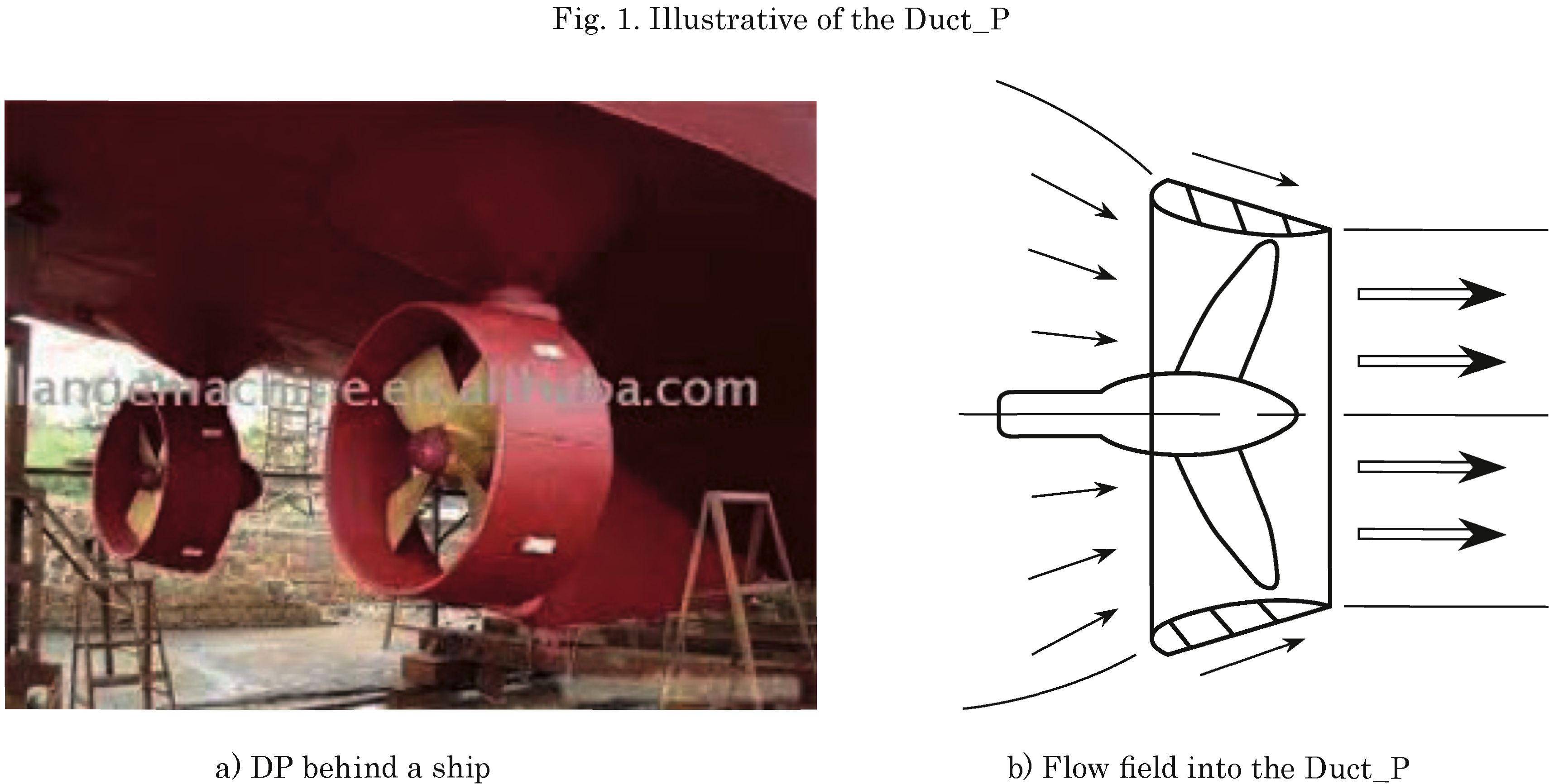
Different types of the marine vessels are widely equipped with ducted propellers (Duct_Ps). Thrust is generated by propellers and ducts which are lifting bodies. The duct surrounds the propeller with a small slope angle. A Duct_P used on the back of the ship and also vectors that flow into the duct and the propeller are shown in Fig. 1. To give more efficiency, it is recommended using Duct_P in ships such as tugs and trawlers (a type of fishing vessel) that work in heavy conditions. Ducts produce thrust augmentation especially in heavy conditions. Generally speaking, it is said that in extreme conditions, the duct may generate 50% of the total thrust. Therefore, it is necessary to focus on the Duct_P to understand that the duct and propeller generate all forces and moments.
(Ghassemi et al.) have carried out the numerical method on the many types of propellers (contrarotating propeller, podded draive, surface piercing propeller and ducted propeller). Many researchers have conducted various experimental and numerical approaches on Duct_Ps. (Haimov et al. 2010) carried out the prediction calculation method using the RANSE code to calculate the open water behavior of the Duct_P. (Kerwin et al. 1987) have used a combination of BEM to model the duct and a vortex lattice method (VLM) for the propeller. The most popular choice in Duct_P numerical studies has been
the RANSE method coupled with an isotropic turbulence model like the SST k-co model, i.e. employed by (Menter 1994).
(Pangusión 2005) has developed the design of a Duct_P and model tests of a fishing research vessel. (Falco 1983) conducted a study about the analysis of the performance of Duct_P in axisymmetric flows. A RANS-based analysis tool for Duct_P systems in open water conditions was presented. (Zondervan et al. 2006) carried out a study on the flow analysis, design and model testing of Duct_P. Using a vortex lattice and finite volume methods, (Gu & Kinnas 2003) modeled the flow around a Duct_P. (Broglia et al. 2013) analyzed different propeller models and their effect on maneuvering prediction. (Bhattacharyya et al. 2015) conducted a study on the hydrodynamic characteristics of open and Duct_Ps by transitional flow modeling. (Bosschers et al. 2015) were the scholars who conducted the study in open water conditions and they applied a combination of the RANS and BEM to study the Duct_Ps. (Duhhioso et al. 2013, 2014) analyzed the performance of a four blade propeller INSEAN E779A model in oblique flow using CFD code in two load conditions and various oblique angles. (Yao 2015) researched the hydrodynamic performance of a marine propeller in oblique flow. (A. Vega and D.L Martinez 2015) used computational fluid dynamics to conduct a bollard pull test for a double propeller tugboat. They simulated a bollard pull test for a specific
tugboat and evaluated the results with the real test results to which it was subjected after construction.
In this study, the performance of a rotating Duct_P set at two oblique angles (10 and 20 degrees) with respect to the inflow is researched by means of an approach based on the RANSE numerical solution. This propeller type may help to improve the maneuvering of the ship. The selected propeller is the four bladed Kaplan type with 19A duct and the experimental data was obtained from (Carlton 2013).
Methodology
In this paper, the propellers rotational velocity of the propeller is imposed bymodeled using aa moving reference frame (MRF) applied to the inner region of the domain because of the high speed and accuracy of computing and simulating. The MRF is a relatively simple, strong, and efficient, CFD modeling method to simulate rotating machines. Given that the fluid flow becomes stable and transient after times a period of time and using MRF is often meaningful significant in this kind of flows, this frame was applied. In the case event of unsteady flows and when MRF is being used, the CFD codes like such as ANSYS CFX and Fluent may solve the unsteady flow. In this situation, it is necessary to add unsteady terms to all the governing applicable transport equations. The finite volume method (FVM) is used to discretize the governing applicable incompressible Navier-Stokes equations, the finite volume method (FVM) is used while in the hybrid SST-Kco turbulence model is chosen for the case of the numerical treatment of turbulence. The SST-Kco model, introduced by Menter (1994), is more accurate and reliable for a wider class types of flows since it combines the robust and precise formulation of the k-co model in the near-wall region with the free stream independence of the k-s model in the far field.
Continuity Equation
Continuity of Flow, as one of the key principles used in the analysis of uniform flow, is the result of the fact that mass is always conserved in fluid systems without taking into consideration the pipeline complexity or direction of flow. Euler proposed the following basic law of fluid:
In cases where fluid flow is transient, the applicable equations must be discretized in both space and time by implicit and explicit time integration methods. In order to control volumes that do not deform in time, the general conservative approximation of the transient term for the nth time step is:
Numerical Implementation and Results
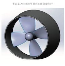
Since has a higher efficiency than a propeller with a normal blade outline when operating in a duct, it is the most common propeller for Duct_ Ps. Having a large chord at the tip is one of the physical characteristics of a Kaplan type propeller. The Kaplan propeller with a P/D ratio of 0.8 is used in the entire analysis of this paper. Geometric modeling of a Kaplan propeller was done with Propcad and Solidworks software. Kaplan geometric data and Duct is shown in Table 1.
Due to the favorable hydrodynamic characteristics, 19A is the most common accelerator type of duct and when it is used with the Ka propeller series it will be more useful in the designing of Duct_Ps. The ducts’ length is equal to half of the propellers’ diameter (Zp=0.5DP) and the distance between the propellers’ tip and the inner surface of the duct is equal to one percent of the propellers’ diameter

(gap=1%Dp). Fig. 2 shows the three-dimensional model of the Duct_P created in Solidworks.
Mesh Generation and Boundary Conditions
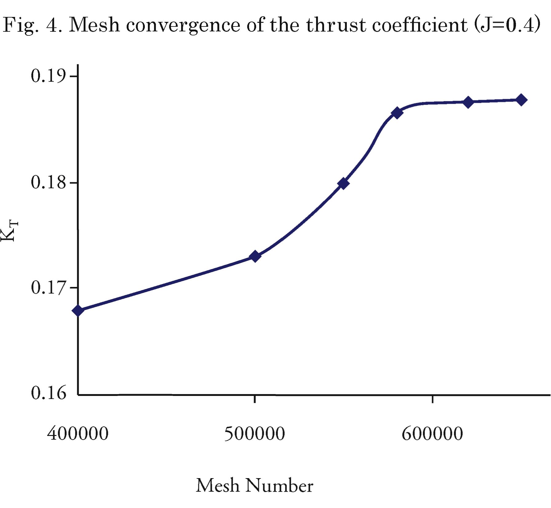
ICEM software is applied to generate unstructured mesh in Duct_P and domains. The generated mesh size grows outwards at a 1.2 ratio. Boundary conditions include inlet, outlet, rotating domain, open water, propeller and duct. Fig. 3 shows the meshes near the propeller and the duct. Due to the complex geometry of the propeller and its gap with the duct, this surface is first divided into seven separate surfaces and a structured quadrilateral surface grid is generated for each one. The average size of the mesh elements on the propellers’ surface at its finest generated mesh is 0.005Dp. Then, this surface mesh is extruded in a wall-normal direction with a transition ratio of 1.1 (for finest generated mesh), an initial layer thickness of 2.5 x 10"5m (corresponding to F = 1) and a layer numbers of n = 50 that results in a streamlined structured hexahedral mesh volume in near-field flow. In the first step, 4 million meshes were used for meshing the model; then, using smaller meshes, 5, 5.5, 6, 6.2 and 6.5 million-cell models were tested and the results were compared at an advanced ratio of 0.4. Comparison of the results shows that the minimum number of cells for this model is 6 million. Fig. 4 shows the mesh convergence of the thrust coefficient. The computational domain consists of an internal rotating cylinder containing Duct_P and an external stationary cylinder with a radius of 1.5D. The inlet uniform boundary condition is located at 3D upstream of the propellers’ plane and the constant pressure condition is imposed at 6.5D downstream.

Also, a second order backward Euler for transient scheme in continuity and momentum equations and upwind method to solve advection turbulence kinetic energy k and specific dissipation rate CO are applied. The SST turbulence model is selected in most of the articles, because of its popularity due to its higher accuracy. Total duration of time is set to 10 seconds and the time steps are selected based on the propellers’ rotating speed for each run.
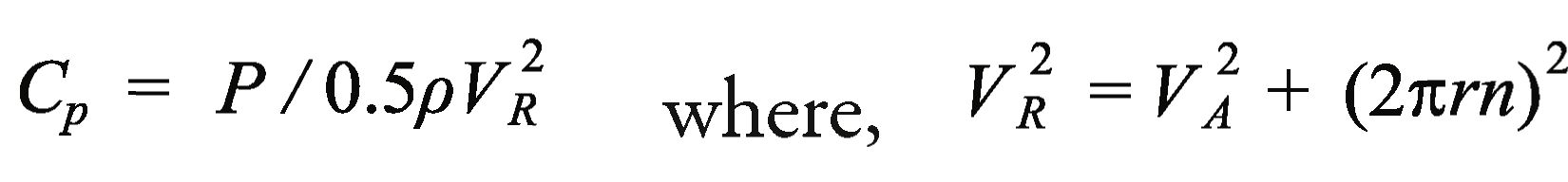
Hydrodynamic performance of Duct_P is defined as follows:
The propeller has been tested for two different advance ratios (/=0.3 and 0.5), covering a relatively
broad set of oblique angles (up to 20). In this numerical simulation, the advance velocity has been kept fixed at a value of 1.5 m/s (12=1.5 m/s) and a rotational velocity of the propeller varied for each condition. The total time duration set to 5s and time steps varied for each advance ratio. Time steps were selected according to the rotational velocity that the propeller would rotate 5o in each time step. For /=0.3 time step was 0.005s and for /= 0.5 time step was 0.0083s. The focus of the numerical results is on forces and moments produced by the Duct_P and the distribution of pressure on the blade and duct.
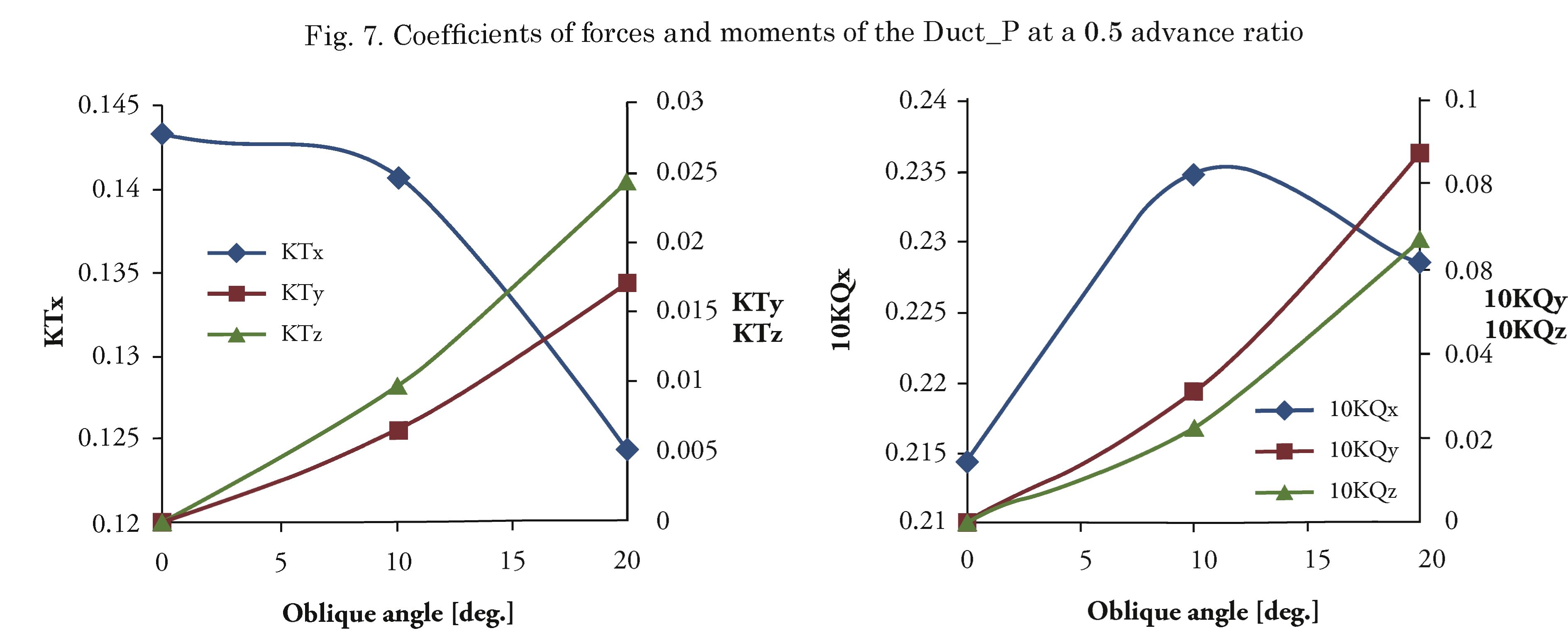
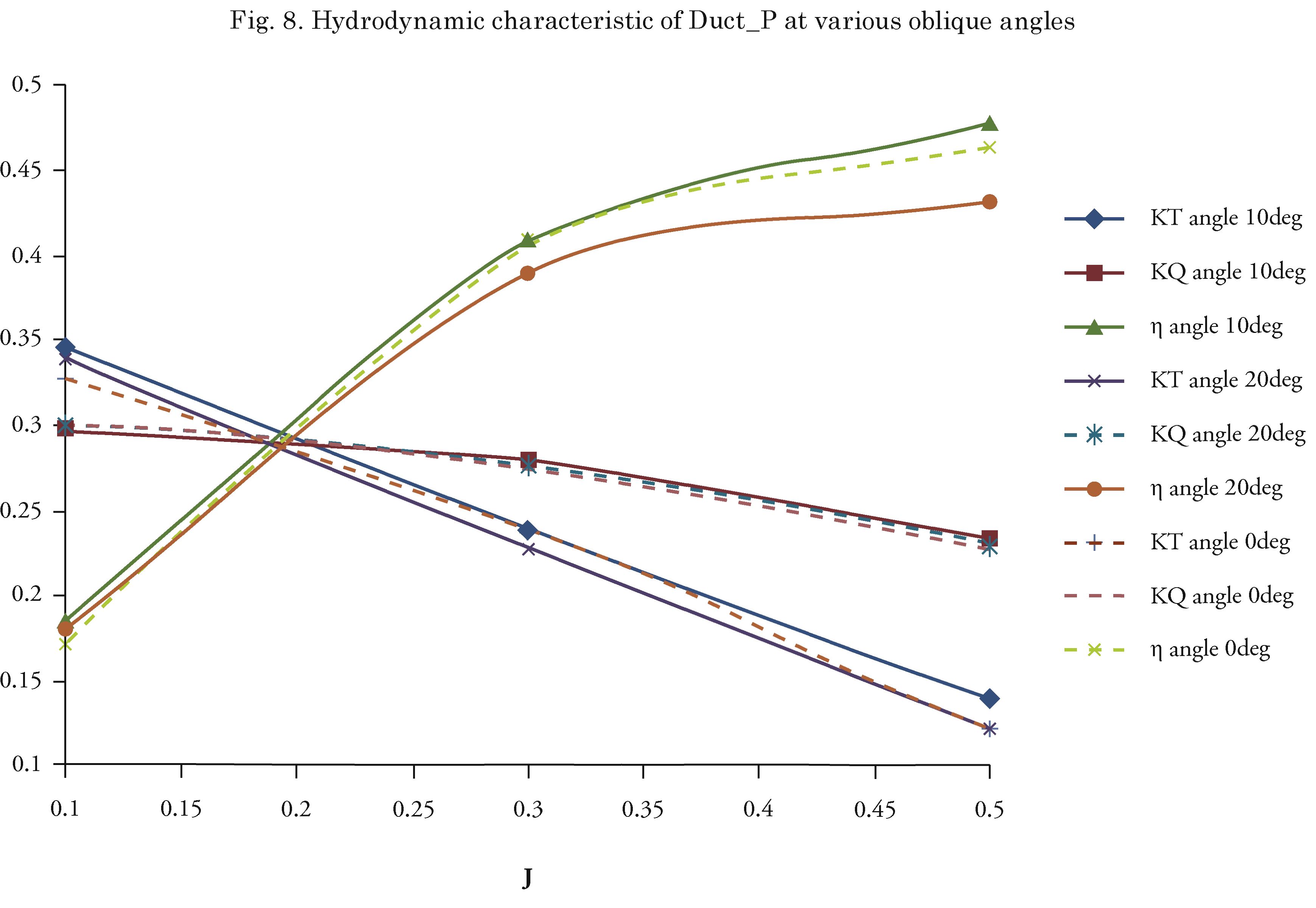
Fig.s 6 and 7 show the coefficients of the forces (KTx, KTy, KTz) and the coefficients of the moments (.KQx, KQy, KQz) against oblique angles of 0°, 10° and 20° degrees at/=0.3 and J= 0.5. The x-component of force (means thrust coefficient KTx) and moment (means torque coefficient KQx) are important and larger than others. When the oblique angle increases, thrust decreases and torque changes are different. Other components increase when the oblique angle increases.
The hydrodynamic characteristics of Duct_P at oblique angles of 0°, 10° and 20° are shown in Fig.

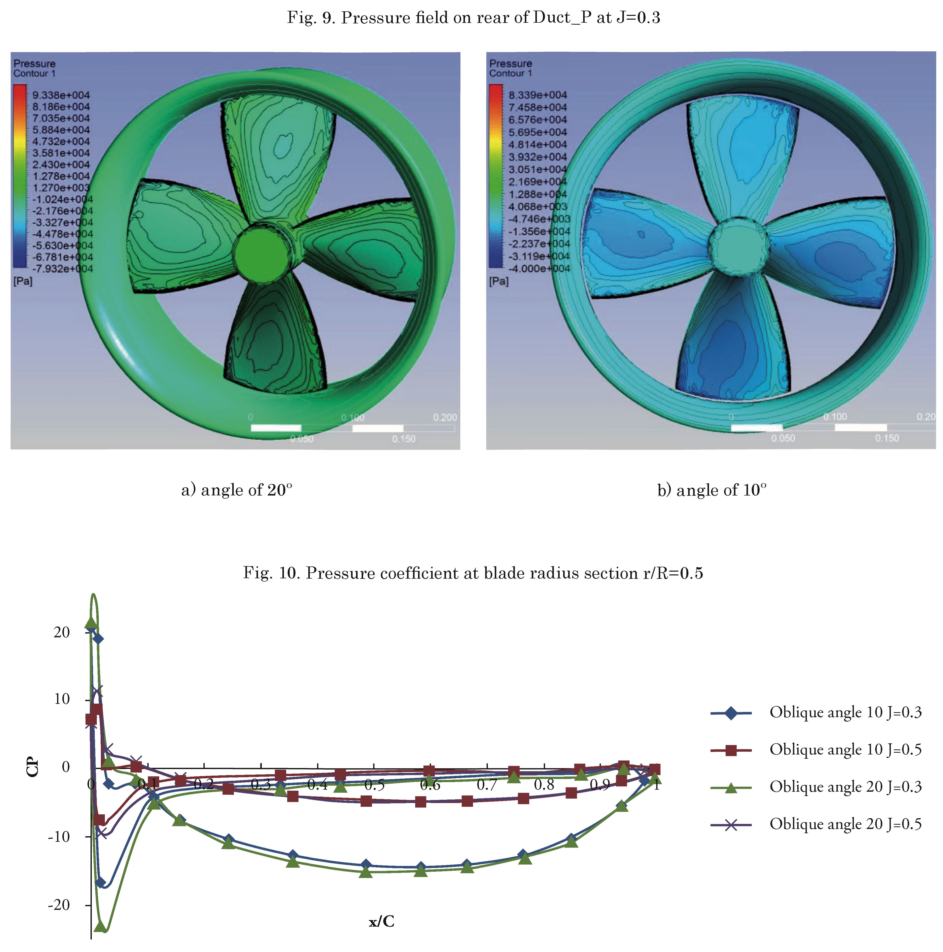
8. The results show that torque does not change when the angels are changed but thrust and efficiency change at all advance coefficients. Fig. 9 shows pressure field on the rear of Duct_P at an advance coefficient of 0.3 for both angles of 10 and 20 degrees. Quantitative comparisons of pressure distribution coefficients
Cp = P/0.5pV2R wherC) vl = V2a + (271
on the propeller blade and duct are presented in Figs. 10 and 11. The results obtained at two advance
ratios (/=0.3 and 0.5), oblique angles of 10 and 20 degrees are shown in Fig. 10. Lower pressure is obtained at the rear of the blade and also on the inner side of the duct. Pressure is almost constant on the outer surface of the duct, while it is low on the inner surface from the leading edge of the duct to x/C= 0.55 (middle length of chord) because in this part, the pressure can decrease alot due to the rear side of the propeller. Cavitation happens at the most time in this part. For this reason, special materials should be used to prevent erosion.
In this article, the Kaplan propeller with duct 19A is analyzed at two advance ratios of 0.3 and 0.5 by the numerical method in open water and oblique flow conditions (10 and 20 degrees). The following results can be drawn:
• Hydrodynamic performance of Duct_P is compared with the experimental data and shows good correlation at high advance coefficient but some discrepancy at low advance coefficient.
• Pressure distributions are obtained on the propeller blade and duct. Low pressure and high pressure are at the rear side of the blade and duct.
• Hydrodynamic performances of the Duct_P are compared at oblique angles (10 and 20 degrees). When oblique angle increases torque does not change, while efficiency significantly changes especially at high advance coefficients.
Greater understanding of the flow at the propeller downstream and the other oblique angles is required. This is a research area that the authors intend to pursue in more detail in the future.

Acknowledgment
Numerical computations presented here have been performed on the parallel machines of the High Performance Computing Research Center (HPCRC) of Amirkabir University of Technology; their support is greatly recognized.
different turbulence models,” American Journal of Mechanical Engineering A. (5), 169-172.
Dubbioso G., Muscari R., Mascio A.D., “Analysis of the performances of a marine propeller operating in oblique flow,” in Computers & Fluids, 75, April 2013, pp.86-102.
References
Bhattacharyya A., Neitzel J.C., Steen S., Abdel-Maksoud M., Krasilnikov V., , “Influence of flow transition on open and ducted propeller characteristics,” Fourth International Symposium on Marine Propulsors, Austin, Texas, USA, June, 2015.
Bosschers J, Willemsen Ch., Peddle A., Rijpkema D., “Analysis of ducted propellers by combining potential flow and RANS methods,” Fourth International Symposium on Marine Propulsors, pp.639-648, Austin, Texas, USA, June, 2015.
Broglia R, Dubbioso G, Durante D, Di Mascio A., “Simulation of turning circle by CFD: analysis of different propeller models and their effect on maneuvering prediction,” in Applied Ocean Research, 2013, 39(1), pp.1-10.
Carlton J. S., “Marine propellers and Propulsion,” 2013, Third edition, Elsevier Ltd.
Dubbioso G., Muscari R., Mascio, A. D., “Analysis of a marine propeller operating in oblique flow. Part 2: Very high incidence angles,” in Computers & Fluids, 92, March, 2014, pp. 56—81.
Falcao de Campos, 1983, “On the calculation of ducted propeller performance in axisymmetric flows,” PhD Thesis, Delft University, Wageningen, The Netherlands.
Ghassemi H., Taherinasab M., 2013, “Numerical calculations of the hydrodynamic performance of the contra-rotating propeller (CRP) for high speed vehicle,” Polish Maritime Research, 20(2), pp.13-20.
Gu H and Kinnas S A., “Modeling of contrarotating and ducted propellers via coupling of a vortex-lattice with a finite volume method,” in Proceedings of Propeller/Shafting Symposium, SNAME, Virginia Beach, USA, 2003.
Haimov H., Bobo M. J., Vicario J., and Del Corral J., “Ducted propellers; a solution for better propulsion of ships, calculations and practice,” in Proceedings of the 1st International Symposium on Fishing Vessel Energy Efficiency, Vigo, Spain, 2010.
Hoekstra, M., “A RANS-based analysis tool for ducted propeller systems in open water conditions,” International Shipbuilding Progress 53, 2006, pp. 205-227.
Kamarlouei M., Ghassemi H., Aslansefat A., Nematy D., “Multi-objective evolutionary optimization technique applied to propeller design,” Acta Polytechnica Hungarica, 2014, 11(9).
Kerwin J. E., Kinnas S. A., Lee J. T. & Shih, W.Z., “A surface panel method for the hydrodynamic analysis of ducted propellers,” Transactions of Society of Naval Architects and Marine Engineers, 1987, 95.
Majdfar S., Ghassemi H., Forouzan H., “Hydrodynamic Effects of the Length and Angle of the Ducted Propeller,” in Journal of Ocean, Mechanical and Aerospace—Science and Engineering Vol. 25.
Menter, F. R., “Two-equation eddy-viscosity turbulence models for engineering applications,” in AIAA Journal, 32(8), 1994, pp. 1598-1605.
Shamsi, R. Ghassemi H., “Time-accurate analysis of the viscous flow around puller podded drive using sliding mesh method,” in Journal of Fluids Engineering, 2015, Volume 137 / 011101-1.
Vega A. and Martinez D.L, , “Reenactment of a bollard pull test for a double propeller tugboat using computational fluid dynamics”, in Ship Science & Technology, 2015, Vol. 8, no. 17, pp. 9-18.
Yari E., Ghassemi H.„ “Hydrodynamic analysis of the surface-piercing propeller (SPP) in unsteady open water condition using boundary element method,” in International Journal of Naval Architecture and Ocean Engineerings 2016, Volume 8, pp. 22-37.
Zondervan, G-J., Hoekstra, M. & Holtrop, J., “Flow analysis, design and testing of ducted propellers”, Proceedings of Propeller/Shafting Symposium, Virginia Beach, United States, 2006.
Yao J., “Investigation on hydrodynamic performance of a marine propeller in oblique flow by RANS computations,” in International Journal of Naval Architecture and Ocean Engineering 2015, 7(1), Pp56-69.