
Ship Science & Technology - Vol. 16- n.°32 - (55-74) January 2023 - Cartagena (Colombia)
DOI: https://doi.org/10.25043/19098642.133
Alejandro Luna García-Valenzuela1
Izak Goedbloed 2
1 Damen Naval, The Netherlands. Email: A.Luna@damennaval.com
2 Damen Naval, The Netherlands. Email: I.Goedbloed@damennaval.com
Date Received: November 25th, 2022 - Fecha de recepción: 25 de noviembre de 2022
Date Accepted: January 20th, 2023 - Fecha de aceptación: 20 de enero de 2023
Navy vessels are relative long and slender ships which must withstand, during their extensive operational life, cyclic loads produced by the seaway. Fatigue is, hence, for those vessels a dominant parameter in the structural ship design and on their operation. Due to the arising complexity of fatigue assessments, an in-house tool is developed to perform automatized spectral fatigue analysis. Tool is called SEAFALT and stands for Long-Term Spectral Fatigue Analysis. This article described the calculation process of SEAFALT, together with results of a case of study. SEAFALT controls automatically the coupling process of the hydrodynamic load calculated on each sea scenario (via ANSYS AQWA), with its correspondent Finite-Element (FE) structural response (via ANSYS MAPDL). SEAFALT calculates: the expected longterm fatigue damage on each node of the FE-model and the minimum required FAT-class.
Key words: Fatigue, Spectral Analysis, Ship Structures, Stress RAO’s, ANSYS, MAPDL, AQWA, Pyansys, Damage.
Los buques militares son barcos relativamente largos y esbeltos que deben soportar, durante su extensa vida operativa, las cargas cíclicas producidas por el mar. La fatiga es, por lo tanto, para esos buques un parámetro dominante en el diseño estructural del buque y en su operación. Debido a la creciente complejidad de las evaluaciones de fatiga, se desarrolla una herramienta interna para realizar análisis de fatiga espectral automatizados. La herramienta se llama SEAFALT y significa Análisis de Fatiga Espectral a Largo Plazo. Este artículo describe el proceso de cálculo de SEAFALT, junto con los resultados de un caso de estudio. SEAFALT controla automáticamente el proceso de acoplamiento de la carga hidrodinámica calculada en cada escenario de mar (a través de ANSYS AQWA), con su correspondiente respuesta estructural de elementos finitos (FE) (a través de ANSYS MAPDL). SEAFALT calcula: el daño por fatiga esperado a largo plazo en cada nodo del modelo FE y la clase FAT mínima requerida.
Palabras claves: Fatiga, Análisis Espectral, Estructuras Navales, RAO’s de tensión, ANSYS, MAPDL, AQWA, Pyansys, Damage.
Damen Naval (DN) is specialized on the design of naval ships and complex commercial vessels. Navy vessels are relative long and slender ships which must withstand, during their extensive operational life, cyclic loads produced by the seaway. This process triggers the formation of cracks at the structural welds which may reduce the capacity of the structure against further load scenarios. Fatigue is, hence, for those vessel types a dominant parameter in the structural ship design and on their operational usability.
During the last years, DN has been confronting more and more with new requirements for ship fatigue lifetime calculations. Such requirements must be implemented on the ship structural design, which in majority of the cases, due to the complexity of the calculations, requires a major engineering effort. Therefore, to deal efficiently with fatigue assessments on engineering phases approximations and simplifications must be accounted, according to International Recognized Standards.
Nowadays, thanks to the growth of computational power, such approximations can be even implemented in software and/or tools throughout which (even more) complex calculations can be performed, allowing engineers to predict the behavior of the ship’s structure on a (more) reliable way.
Hence, to assist structural analysts along the engineering phases on fatigue assessment, it was developed SEAFALT, a software-tool (script) able to perform automated spectral fatigue assessments to establish the coupling between the pressure distribution (calculated on each evaluated sea scenario) with its consequent Finite-Element (FE) structural response (Luna Garcia-Valenzuela, 2019). The used seakeeping tool is ANSYS AQWA, while the chosen FE-software is ANSYS MAPDL (Mechanical APDL). The complete automated process is controlled by a Python-script that was called SEAFALT (LongTerm Spectral Fatigue Analysis).
Fatigue occurs as a result of stress or strain reversals, known as cycles, in the time history. It therefore sets the response of the structure or component as the starting point for any fatigue analysis.
Fatigue damage has been traditionally determined from time signals of loading, usually in the form of stress or strain. Such methodology is suitable for periodic loading, nevertheless requires large time records to accurately describe random loading processes. The offshore oil industry faced this problem in the early 1980’s, since the offshore platforms are large and complex structures subj ected to random wind and wave loading. The analysis becomes complicated because the imposed loads are random and excite dynamically the structure, proving this way the transient dynamic analysis in the time domain as unfeasible (Halfpenny, 1999). On the other hand, for many FE analyses (especially when modelling dynamic resonance), a compact frequency-domain-based fatigue calculation can be utilized alternatively, where the random loading and response are categorized using Power Spectral Density (PSD) functions, and the dynamic structure is modelled as a linear transfer function. In fact, it is often beneficial to carry out a rapid frequency response (transfer function) analysis instead of a computationally intensive transient dynamic analysis in the time domain (Halfpenny, 1999).
Therefore, a FE analysis based in hydrodynamic frequency-domain loads can simplify the problem severally. Such calculation can then be carried out to determine the transfer function between wave height and stress in the structure. Following this, the PSD of wave height is simply multiplied by the transfer function to obtain the PSD of stress response of the structure.
Fatigue in floating structures is mostly driven by moderate sea states, for which linear analyses often suffice (Naess & Moan, 2013). Therefore frequencydomain analyses of wave-induced response for various sea states can then be efficiently carried out with relatively coarse FE models of the structure, allowing the calculation to be speeded-up in comparison with the time-domain computation. Hence, the calculation of the relevant fatigue loads involves a global analysis and their effects in terms of member forces, and a local analysis to determine the hot spot stress, as illustrated on Fig. 1.
Fig. 1. Fatigue loading in terms of stress ranges. (Naess & Moan, 2013).
The frequency domain is another domain in which to view a time signal but losing the phase information, but now the x-axis represents frequency instead of time. In practice, frequency domain is usually represented as a ‘Power Spectral Density (PSD)’ plot, which consists on a normalized density plot that describes the mean square amplitude of each sinusoidal wave with respect to its frequency. Fig. 2 shows a typical PSD plot, where the mean square amplitude of a constituent sinusoidal wave can be determined by measuring the area under the PSD over the desired frequency range.
Fig. 2. Typical PSD of a random time history. (Halfpenny, 1999).
Frequency Hz
The time signal regeneration is performed throughout an ‘Inverse Fourier Transformation’ on the complex vector of frequency domain results, however, when the starting point is a PSD this method is inappropriate due to the lack of wave phase information of such PSD. However, for certain time stories such as the ‘ergodic stationary Gaussian random processes’, assumptions about the original phase content can be made for the time series to be regenerated. For fatigue assessments in the frequency domain ‘ergodic stationary Gaussian and random’ processes are assumed.
For every occurring sea state, the stress response spectrum (or spectral density function) can be easily obtained within the frequency domain approach. For a narrow-banded Gaussian process, every peak is coincident with a cycle and, consequently, the stress amplitudes are Rayleigh-distributed. Now if the Stress-Cycles curve (SN) is formulated in terms of: N the number of cycles to failure for stress range S, m the negative inverse slope of the SN curve and K - factor the slope of the curve which governs the relationship between the stress level and the number of cycles, as:

then the expected fatigue damage D is:

where NT is the total number of stress cycles, S is defined by  , and E[] denotes the expectation value operator. S may be interpreted as a constant amplitude loading that is equivalent to the random loading under the assumption of a single slope SN curve.
If the described Gaussian process has zero mean and variance  , the stress range follows a short term Rayleigh distribution, and can be determined from the stress amplitude distribution fA:

The short-term fatigue damage can be therefore expressed as:

with Γ(;) the Euler gamma function.
To perform the long-term fatigue assessment, all or at least the most contributing sea states must be accounted. Long-term fatigue damage can be expressed, in terms of Rayleigh short-term distributed stress ranges, as indicated below (DNVGL, 2015):

where rinj is the relative number of stress cycles in short term condition i, n for loading condition j, aj is the probability of loading condition j, nLC is the total number of loading conditions and m0inj is the zero spectral moment of stress response process in short term condition i, n and loading condition j.
On the other hand, if bi-linear SN curves are to be used, according to (DNVGL, 2015) they can be expressed logarithmically as:

where δ is the standard deviation of logN, and K1, K2 are the constant of mean SN curve (50% probability of survival) and the constant of design SN curve (97.5% probability of survival), respectively. With this, Eq.5 can be expressed as:

with Δσq the stress range in SN curve, where the change of slope occurs (knuckle), K2, m are the SN fatigue parameters for N<107 cycles, K2= m + Δm are the SN fatigue parameters for N>107 cycles. SN curves are generally designated by DNVGL with FAT X, where X is the stress range at 2·106 cycles.
For floating structures, the (Morison's) drag force implies super harmonic load components that are normally an order of magnitude smaller than the wave frequency component. However, if the higher-order harmonic load components coincide with the natural frequency, significant amplification occurs, making the high-frequency load effect significant. Slamming and sloshing in tanks can similarly contribute in fatigue loading. This means that the stress history comprises a high- and low-frequency response process and therefore becomes wide banded (Naess & Moan, 2013). As the shape and the variance of the stress-range-response spectrum has a significant effect on the prediction of the induced fatigue damage, a correction factor can be used to consider the band-wideness of the process. Benasciutti and Tovo (2005) proposed an empirical formula of wide-band fatigue damage by using a linear combination of the narrow-band and range counting results that can be obtained by closed-form expressions in the frequency domain:

where m is the material parameter of the SN curve, DNB is the fatigue damage under the narrow band assumption, fBT is the Benasciutti-Tovo correction factor, and the coefficient b is empirically obtained based on extensive numerical simulations. This (8) formula has been shown to give accurate results in an independent study (Gao & Moan, 2008), and therefore can be applied with good accuracy to all types of wide and narrow band Gaussian processes (Naess & Moan, 2013).
SEAFALT is meant to be used during a basic engineering phase allowing the user to compute the minimum required characteristics of structural details, to ensure the withstanding of the variety of sea loading cycles during the vessel operation. It could be also used during detail engineering phases to determine the lifetime of the structure, once it has been designed. Fig. 3 shows the logo of SEAFALT.
Fig. 3. SEAFALT Logo.
The development of this tool, was driven by the following key needs:
Spectral fatigue analysis is fast, in a lot of cases accurate and, more important, a closed form method (Zurkinden, A. et al., 2014). The aim of the spectral analysis is the determination of the long-term fatigue damage with a direct calculation approach that takes into account the different environmental conditions encountered by the floating structure. So, the core of the analysis is the determination of a Response Amplitude Operator (RAO) between the waves and the stress, for each operating condition. This RAO is obtained by the combination of a frequency-domain-based hydrodynamic model with a linear structural model. Although different hydrostructure coupling schemes are available, it was chosen the process-flow proposed by Bureau-Veritas (Veritas, 2016), as shown in Fig. 4. It is widely used and is based on transferring the wave loads from the hydrodynamic model on a three-dimensional FE model for each wave heading, frequency and speed.
Fig. 4. Spectral fatigue analysis flowchart (Veritas, 2016).
Using the stress RAO, a stress response spectrum can be determined for each wave energy density spectrum. Providing short-term wave statistics and considering the fatigue capacity given by the SN curve, a shortterm damage is calculated. Finally, the long-term fatigue damage is computed as the summation of short-term damages taking the probability of occurrence of each sea state into account.
This method allows for short computational times as well as a for a direct spectral analysis of the accumulated damage in a given structural detail. On the other hand, the method does not allow for the integration of non-linear effects such as the non-linear hydrostatic force or the non-linear drag forces. To account for such effects a time domain simulation remains necessary. However, as fatigue in floating structures is mostly driven by moderate sea states, a linear analysis often suffice (Naess & Moan, 2013).
The developed tool controls the solution, pre- and post-processing of the results from the different solvers or modules used to carry out the spectral fatigue analysis of the structure: ANSYS-AQWA and ANSYS-MAPDL. SEAFALT therefore acts as the “glue” of the complex data management of this process: handling inputs, moving, processing, sending and storing data from the different solvers involved. The calculation flow is then composed by four subprocesses:
Determines the wave excitation transfer function for different incident wave angles, wave frequencies and ship speed. For the given operational profile, the wave induced load is obtained at a given location per unit wave amplitude, by computing the pressures and rigid body motions of the center of gravity of the structure throughout a linear-diffraction analysis. Response X of a structure subjected to wave loading is therefore calculated by solving the equation of motion in the frequency domain for unit wave amplitude.
In this step, the stress transfer functions (STF) or stress Response Amplitude Operator (RAO) are determined by applying the calculated hydrodynamic loads on a 3D FEM structural model. The STF expresses the relationship between the stress at the given structural location and a unit wave amplitude. The procedure is based on computing the linear structural response of the imported hydrodynamic load scenarios. This is done by means of the integration of the pressure values within panels, allowing for the calculation and transfer of discretized loading values inside the same panel, to the detailed FEM mesh. Hence, for each wave frequency ω, heading θ and ship speed v, the hydrodynamic load case scenario is solved via a FEM static structural simulation, and from nodal stress results the stress transfer function HΔσ (ω|θ|ν) is obtained. Fig. 5 summarizes graphically the intermediate results of the process to calculate the stress range response. To compute fatigue damage, the effective stress range is computed at each shellelement node of the structural model (DNVGL, 2015), since accounts for the situation with fatigue cracking along a weld toe, but also when principal stress direction is more parallel to it.
Fig. 5. Curves used on the computation of the stress range response: STF (RAO), Sea Spectrum and Stress Response (from left to right).
Once all load cases are solved, the STF data base is consolidated, from which short-term stresses can be calculated spectrally for different irregular seaway scenarios described in the operational profile.
This module calculates the long-term fatigue damage or the minimum required FAT class, at a certain evaluated node of the structural model. To do that, first the short-term stress (range) response spectrum SΔσ is calculated for sea states described in the operational profile, by accounting for sea spectrum SF(ω|θ) and the respective STF, previously determined.

Then, the spectral moments are calculated by means of the following expression:

Now Benasciutti-Tovo correction factor (Eq. 9) is determined. And finally, when all the sea conditions are evaluated (repeating the above described process), the long-term fatigue damage equation (Eq. 8) is solved. subroutine classifes the nodes on evaluation in: base-material, welds and free-plate edge (see Fig.6), for which one reference FAT-class (SN Curve) is assigned according to DNVGL (2015).
Fig. 6. Nodal and element classification: (from left to right) elements attached to weld nodes, base material nodes, and free-plate edge nodes.
Solving Eq. 8 can be done in two different manners, depending on the type of fatigue assessment:

Long-term damage (Fig. 8), in which the actual FAT-class of the evaluated structural detailed is known, respective SN-curve parameters are introduced and the equation is solved straight forward.

The developed calculation process was tested with a full scale detailed (FE) model of a pontoon-barge designed and built by DAMEN (Fig. 9).
Fig. 9. Pontoon vessel used as study case. (Damen, 2019).
The method to assess global hull-girder structural response is applicable to various hull-shapes, including military-ships. On the other hand, the curved shape of the hull could trigger the buoyancy forces to vary non-linearly with the wave height, inducing weak-nonlinear seakeeping behavior. As the proposed methodology is based on linear hydrodynamics, this non-linear phenomena might not be possible to be directly captured by the seakeeping tool. However as stated in III-C a linear hydrodynamic analysis often suffice for fatigue loading assessments, due to the fact that the expected hydrodynamic response at the recommended rule-based probability of exceedance shows normally a linear trend (DNVGL, 2015). Hence, and for simplicity reasons the abovementioned barge was chosen as a case of study.
The pontoon is a (relatively simple) barge, with vertical bulkheads and shell, a block coefficient nearby the unit, for which fatigue issues are not expected to appear during its lifetime considering the mild operational profile. The simplicity of the geometrical model to be used in the calculation was hence considered. Main dimensions and hydrostatics of the pontoon model can be summarized in Table 1.
Table 1. Main Particulars and Hydrostatics of the Pontoon model.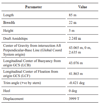
In this section the two models used on the computation are described: hydrodynamic and FE model.
The model used during hydrodynamic simulations consists of a 3D outer-hull-plating model (Fig. 10). Mass and inertia properties are represented through a single mass point with the following characteristics:
Fig. 10. Hydrodynamic Model of the Pontoon.
Reader can note that the vertical coordinate of the CoG stated at Table 1 and Table 2 differ from each other. This occurs due to the fact that the origin of the Global Coordinate System of the hydrodynamic model does not coincide with the one of the FE model. The difference is corrected automatically when the coupling is performed.
Table 2. Mass point properties.
The maximum element size of the panels was set to 3 meters, with a defeaturing tolerance of 0.8 m. With it, it was possible to evaluate wave frequency ranges from 0.25 rad/s to 1.8 rad/s with 50 intermediate values. Different wave heading directions were assessed, from 0 to 180 degrees with steps of 30 degrees. Regarding the pontoon speed, three values were evaluated: 3, 9 and 12 knots.
To carry out FE calculations, a fine mesh of around 256.000 nodes were used to discretize the structure of the pontoon.
Figs. 11 and 12 shows the geometry of the pontoon, which was modeled by using the following element types:
Fig. 11. Pontoon FE Model.

In the corners of these holes, high concentration of stresses is expected which will likely create longterm fatigue issues.
To create fatigue-sensitive locations in the structure, the main deck plating of the structure was penetrated with four different types of holes, as shown in Table 3 and Fig. 13.


Finally, boundary conditions (Fig. 14) were applied to the model so that it can freely deform while keeping the model numerically balanced:
Fig. 14. Boundary conditions.
Following the process described in Section III-C, the minimum required FAT-class for all the structural nodes in the FE model of the pontoon was calculated.
To do that, the following settings were accounted:
o Base material: Curve B1.
o Free-plate edge: Curves B, B2, C, C1, C2. o Weld: Curves D, E, F.

A total of7224 sea scenarios were evaluated by means the described methodology. As an example, the load transfer method is shown in Figs. 15, 16 and 17.
Fig. 15. Wave Loading on FEM Model. Contour-plot of applied pressures.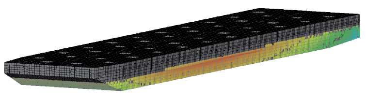


The arrow's length and color give an idea of the magnitude order. The sign of the pressure value in the legend shows the direction of the pressure vector: positive pressures are applied against the element centroid while negative ones are applied outwards from the element surface. The mid-ship section of the pontoon is situated at the wave crest while the aft and forward region are located at the trough of the wave. Moreover, it can also be noted that the free surface is not perfectly read as a straight line, depending it on the number of elements used on this region of the FEM model. The same applies to the hydrodynamic model and considering the volume calculated through this element discretization, it can be understood that the model will never be completely balanced with regards to the hydrostatic loads. As the calculated volume through elements will be smaller than the actual one, the buoyancy force will be then smaller than the actual weight of the vessel. Therefore at boundary-condition nodes residual stresses and reactions are expected to appear.
Reactions at boundary-condition nodes were monitored. For the worst scenario, the sum of the vertical reaction forces at such nodes was -5.32 kN (0.01% of displacement), thus can be considered that the model was properly balanced.
After the full computation was completed, outputs were analyzed qualitatively, due to the complexity on evaluating long-term results. Intermediate steps were studied and verified (Luna Garcia-Valenzuela, 2019). Quantitative assessment will follow in future work. Results were mapped over the FE model. The following plots were generated:
As shown in Fig. 18 and Fig. 19, in the aft- and forward-end regions the minimum required stress range at 2·106 cycles is small (almost 0 MPa) in comparison with the mid-ship region of the vessel, where the minimum required FAT-class for the nodes is about 35 MPa. This structural response was completely expected, due to the mild operational profile. Structural fatigue is known to be dominated by the vertical induced wave bending moment. As the transversal second moment of inertia is higher than the vertical one, then it proves that the transversal bending moment (inversely dependent of the second moment of inertia) is much smaller than the vertical wave bending moment. Consequently, the transversal stress on the structure will be also smaller than the longitudinal stress, therefore setting the importance of the longitudinal stress on fatigue assessment.
Fig. 18. Minimum Required FAT-Class (Automatic Coloring Scale): Overview.

Being the extremes of the pontoon constrained by the boundary conditions, the most unfavorable condition will be the case in which the wave peak is located at the longitudinal position of the center of gravity, and the wavelength is equal to the pontoon length on head seas. This was the case shown in Fig. 15 where the maximum vertical bending moment occurred in the middle of the vessel. Therefore, it can be understood that the part of the structure in which it is expected to exist fatigue issues it is the midship region of the vessel. This behavior can be also shown in Fig. 20, where the higher minimum required FAT-class again appears on the nodes located at midships. Fig. 19 also shows the expected stress distribution among the different structural members.
Fig. 20. Minimum Required FAT-Class (Automatic Coloring Scale): Overview without deck plating.
In Fig. 21, it is shown on a profile-view the same minimum required FAT-class distribution evaluated previously. Here, it can be noted that in the line of the neutral axis, there is almost no longitudinal stress. This fact triggers that this zone, not only in the hull plating but also in nodes which are nearby the neutral axis line of longitudinal bulkheads, have a low FAT-class requirement. Similarly, in the same view it can be noted that in the deck and bottom regions, minimum required stress range is higher due to the fact that they are subjected to bending moments, which are more significant, as commented, the bigger distance of the neutral axis (in vertical direction) and the closer to the midship region (in longitudinal direction).
Fig. 21. Minimum Required FAT-Class (Automatic Coloring Scale): Profle view
Fig. 22 shows the minimum required stress range distribution throughout the main-deck platting of the pontoon. First, it can be noted again the same behavior described previously with regards to the required FAT-class at midships. This response in addition to the effect caused by the structural holes will increment notably the required stress ranges around the edges of such holes. Penetrations consist basically in structural discontinuities which interrupts the stress flow within the plating. That forces the stress to flow around the hole. That will result in stress concentrations around the discontinuity edges.
Fig. 22. Minimum Required FAT-Class (Automatic Coloring Scale): Plan view.
In Fig. 23, this effect can be noted easily since it is a zoom-in of Fig. 22. Here it can be observed the stress shadows of the holes (blue colored), where the stress concentration is severely reduced, due to the stress direction towards the hole corners, defining therefore the preferable or allowable areas for deck plating penetrations.
Fig. 23. Minimum Required FAT-Class (Automatic Coloring Scale): Plan-detailed view of deck-platting holes
In the squared discontinuities, the stress-flow deviation is bigger than in the one with rounded corners. This effect will increase even more the stress concentration around the squared corners. Red colors therefore arise in the corner edges while only yellow color appear in the rounded corners of the discontinuity.
Fig. 24 shows that none of the nodes of the structure are expected to show fatigue issues during the lifetime of the pontoon, for the considered operational profile. The scale of the figure refers to the stress-range limits of the SN curves (FATclasses), as defined by DNVGL. The general idea of this plots is checking that the actual FAT-class of the designed detail is equal or higher than the minimum required FAT-Class, for the same detail. Thus, if for instance a node of the structure is classified as base material (SN Curve: B1, FAT-160) and in the plots it is colored in red (FAT-160 threshold), it shows that the minimum required FAT-class falls nearby the limit. Similarly, if a node is classified as FAT-71 weld and has a minimum required FAT-class of 112 MPa, it will be colored in green and therefore, the structural detail should be re-designed since is expected to show fatigue issues. If the structure is then completely painted in dark-blue (FAT-Class below 80) it means that the minimum required FAT-class is below the limits defined of the SN curves and no fatigue problems will be expected.
Fig. 24. Minimum Required FAT-Class (FAT Coloring Scale): Overview.
It should be noted by the reader that if more extreme load cases would have been evaluated, probably different parts of the structure would have been facing fatigue response issues, triggering then such parts to be painted in different color than dark blue.
Finally, Fig. 25 shows the expected stress concentration at boundary conditions. It occurs due to the lightly unbalanced buoyancy forces, creating small non-zero reaction forces at these nodes (and also due to the stress distribution, on surrounding nodes).
Fig. 25. Minimum Required FAT-Class (Automatic Coloring Scale): Boundary Conditions.
Through the previous ts, it can be observed the mid-plane symmetry on the response of the structure. In fact, as the geometry and the wave loading are symmetric, it is to be expected that the structural response of the structure will be similarly symmetric. It should be noted that with a different wave phase delay (than 0 degrees) asymmetric wave loading arises and therefore, asymmetric structure response must be expected.
Also the long-term damage computation was calculated. To do that, an unfavorable case in terms of fatigue was created and solved (see Table 5). Long-term damage was calculated for all the nodes in the structure, by solving Equation 8.
Table 5. Sea case of study, for long-term damage evaluation.
As shown in Fig. 27, several locations at strength deck amidships showed long-term fatigue damage above or equal to 1. These structural details were in the majority of the cases welds, for which conservatively the chosen FAT-class was 36, normally used for partial penetration butt-welds (DNV-GL, 2015). Red-marked area around the hatch-hole (Fig. 28) showed a stress range of 270 MPa. Fig. 26 represents the longterm stress range distribution. Accounting for the recommended probability of exceedance level for fatigue assessments, 10-2 (DNV-GL, 2015), and also for FAT36 SN-curve parameters, Equation 8 was solved and the long-term fatigue damage yielded to 1.5. Same value was obtained by the developed tool.
Fig. 26. Long-term stress range distribution of evaluated detail.


This article shows a developed process to perform spectral fatigue calculations for floating structures. Such process is implemented on a software-tool, called SEAFALT, dedicated for spectral fatigue analysis based on a coupling of direct calculated loads and the FE method. Hydrodynamic analyses are based on the frequency domain approach and FE computations are static structural assessments. These facts allow to speed-up significantly fatigue lifetime calculations compared to full timedomain methodologies.
The developed tool is pretended to be used during basic and detailed engineering phases and allows the engineer to compute the minimum required characteristics of structural detail, to ensure the withstanding of the variety of sea loading cycles during the vessel his lifetime. Also, long-term fatigue damage can be assessed, once the detail his characteristics are known.
The spectral fatigue assessment is performed in terms of:
The structure of a pontoon vessel designed and built by Damen DSNS was evaluated through SEAFALT. A full-length-detailed FEM model with 256.000 nodes. Also, a hydrodynamic model was created to evaluate the environmental conditions dictated by the provided operational profile.
For this study, such environmental conditions were quite mild. Hydrodynamically-wise does not trigger the model to develop any fatigue longterm issues, which means that the structure has enough fatigue strength to withstand the potential operational conditions during the entire lifetime and that it has been properly designed. Results were assessed from a qualitative point-of-view and based on engineering experience. Qualitative assessment will be performed in future works. Also future developments will be focused on benchmarking the tool with ships with different hull shapes.
ANSYS, Inc. 2016. ANSYS-AQWA Features. https://www.ansys.com/products/structures/ansys-aqwa/ansys-aqwa-features [Online] 2016.
ANSYS, Inc. 2012. AQWA User Manual. Cyberships. [Online] 2012. https://cyberships.files.wordpress.com/2014/01/wb_aqwa.pdf.
BENASCIUTTI, D. & TOVO, R. 2005. Spectral methods for lifetime prediction under wide-band stationary random process. s.l. : International Journal of Fatigue, 2005. Vol. 27(8), 867-877.
Damen. 2016. Pontoon catalogue. [Online] 2016. https://products.damen.com/en/clusters/ pontoons
DNV-GL. 2015. Fatigue Assessment of Ship Structures. 2015. DNVGL-CG-0129.
HALFPENNY, A. 1999. A Frequency Domain Approach for Fatigue Life Estimation from Finite Element Analysis. s.l. : Key Engineering Materials, 1999. 167-168, 401-410.
LUNA GARCíA-VALENZUELA, A. 2019. Automated Spectral Fatigue Analysis for Floating Structures. Hamburg : Hamburg University of Technology, 2019.
NAESS, A. & MOAN, T. 2013. Stochastic Dynamics of Marine Structures. s.l. : Cambridge University Press., 2013.
Veritas, Bureau. 2016. Guidelines for Fatigue Assessment of Steel Ships and Offshore Units. 2016. NI611 R01.
ZURKINDEN, A., GAO, Z., MOAN, T., LAMBERTSEN, S., & DAMKILDe, L. 2014. Spectral Based Fatigue Analysis of the Wayestar - arm taking into account different control strategies. s.l. : Structural Design of Wave Energy Devices. , 2014.